
Lubos Mitas, Helena Mitasova, William M. Brown, Mark Astley
We propose a computational framework and strategies for performing tasks necessary for evaluation and optimization of land use management within an advanced GIS modeling environment. Such tasks involve modeling of landscape processes, simulation of impact of human activities on these processes and optimization of preventive measures aimed at creating sustainable landscapes. A typical example of interaction between landscape processes and human activity is water erosion, a natural process which can be accelerated or greatly reduced by human intervention. In our implementation, the underlying 2D water and sediment transport equations are solved within approximate diffusive wave hydrologic and detachment/transport capacity models using stochastic methods (Monte Carlo). The methods employ distributed input parameters and enable us to simulate the impact of complex terrain, various soils and land cover changes on the spatial distribution of erosion and deposition. The presented approach together with land use optimization scenario is illustrated by an application to an experimental farm in Germany, carried out within 3D dynamic GIS environment.
This document requires a browser which supports tables.
The full size figures and animations can be retrieved by clicking on
reference images.
Efforts to balance the economic development with environmental protection have increased the demand for simulation tools enabling predictions of the human impact on landscape. In order to prevent irreversible changes and avoid costly, ineffective solutions the simulation tools should provide detailed spatial and temporal distributions of modeled phenomena. Statistical averages for the entire study areas or predictions only for a certain point, such as watershed outlet are often insufficient. New developments in GIS, especially support for multivariate temporal data processing, analysis, and visualization (Mitasova et al. 1995, GRASS4.2 libraries) make such simulations possible and GIS plays an important role in the development and applications of distributed landscape process models (e.g., Engel 1995(review with links), Vieux et al. 1996, Saghafian 1995, Leavesley et al. 1996 ).
The goal of our paper is to outline a methodological framework for distributed models based on the solution of the "first principles" master equations for multi-variate fields and use these tools for the distributed land use scenarios optimization. The basic platforms of our approach are described as follows:
In the following sections we describe the working examples of advanced methods and approaches which enabled us to start from basic input data (terrain, cover, soils, etc) and get to the actual creative process of land use optimization in a fully distributed manner.
The basic objects which enter into distributed models of landscape processes are given by functions which depend on the position in 3D space and time: multivariate scalar and vector fields. These fields represent various phenomena such as terrain, soil properties, land cover, fluxes of matter. They are usually represented in a GIS database in a discrete form as sets of points (sites, lines or polygons) or rasters. However, they can be transformed to continuous representations using expansions in an appropriate basis set such as multivariate regularized spline with tension (Mitasova et al. 1995), as illustrated by examples in Table 1. or by Hargrove et al. (1995). Such representation is not restricted to continuous fields, an example of effective handling of surfaces with faults using splines and GIS tools was developed by Cox et al. 1994. Phenomena represented by classes, such as vegetation or land use, can be represented as fields with faults as well (Table 1., land cover).
Table 1. Examples of landscape phenomena representations
by multivariate fields
( Click on the image to retrieve full size picture or animation)
Representations of natural phenomena as multivariate fields modeled by bi-, tri-, and quad-variate splines | ||||
| phenomenon (field) | 3D (dynamic) "map" | GIS format (discrete representation) | ||
|---|---|---|---|---|
| elevation | 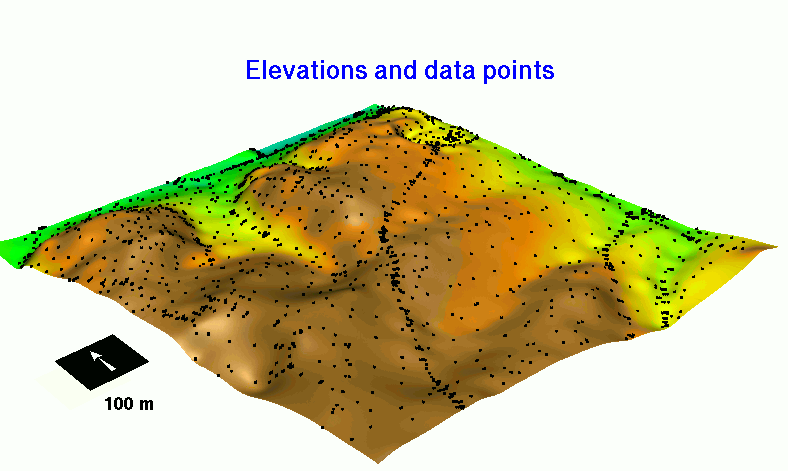 |
points (x,y,z), lines (contours), 2D raster (DEM) | ||
| elevation gradient and curvatures | 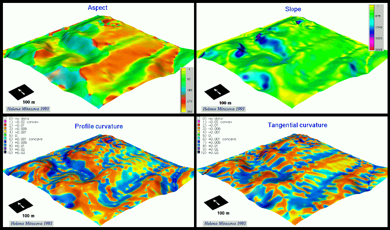 |
2D rasters derived from z=f(x,y) | ||
| precipitation |
 |
points(x,y,z,t,p), 2D raster time series | ||
| soil horizons |  |
points (x,y,z,w), 2D raster vertical series | ||
| land cover | 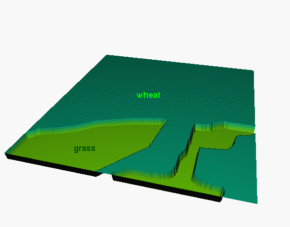 |
polygon, 2D raster | ||
| underground concentrations of chemicals |
 |
points (x,y,z,t,w), 3D raster time series | ||
| concentration of chemicals in water |
 | points (x,y,z,t,w), 3D raster time series | ||
The fields are static or evolving in time. The evolution can be monitored and data from monitoring can be stored in a GIS database in various formats, for example, as time series of sites which can be further transformed to time series of 2D or 3D rasters (e.g., Table 1.,chem. concentrations). To predict the future states of these fields, we need to understand the processes controlling their evolution and formulate models simulating their fundamental behavior. The GIS software is being enhanced to support such simulations by providing the adequate data structures, including 2D and 3D floating point raster data (Waupotitsch and Shapiro 1995), multidimensional site data (McCauley 1995), support for temporal data (Brown and Shapiro 1995), methods for transformation between discrete and continuous representations using multivariate interpolation by radial basis functions (Mitasova et al. 1995), and tools for interactive multidimensional dynamic cartography (Brown et al. 1995).
The problem of landscape process simulations related to land use change have been studied by a variety of approaches, such as rule-based models, cellular automata, probability transitions models, (Berry et al. 1995) or models based on continuous fields and differential equations (Maidment 1996). We use the last approach, with continuous representation of fields and differential equations describing the fundamental conservation laws.
One of the primary processes in landscape, influencing the distribution of soils, plants and people is water flow. While there are numerous empirical and process based models for modeling the water flux in streams and rivers, spatial distribution of water on complex hillslopes (crucial for soils and organisms) is still being modeled by rather rough estimates unable to provide sufficient detail for modeling of some important water related processes, such as erosion.
In general, the overland flow is
described by the continuity equation:

where h is the water depth [m], i is the rainfall
excess=rainfall-infiltration [m/s], q is the water
flux [m.m/s], v is
the flow velocity [m/s],
r=(x,y) is the position [m], and t is the time [s].
The velocity v is related to h by Mannings
or Chezy law and the momentum conservation equation (Haan 1994).
Current GISs provide the tools for the simplest approximate solution of the equation (1) for steady state flow and constant velocity, based on the upslope contributing area. There are numerous algorithms available for its estimation, such as D8 (Figure 1a), or an improved approach based on the vector-grid algorithm (Mitasova et al. 1995, Figure 1b). While these geometric approaches provide enough information for a wide range of applications (Moore et al. 1992), they become problematic when applied to areas with spatially variable cover and complex terrains with significant spatial variations in flow velocity.
A more realistic approximation which takes into account the flow velocity is based on the steady state solution of the equation (1) for the 2D kinematic wave (Figure 1c) and 2D diffusive wave (Figure 1d) approximation (Mitas and Mitasova, in preparation.). The 2D approximate diffusive wave solution can be found by solving the steady state form of the equation (1) written in the operator form as:

 a
a
 b
b
 c
c
 d
d
Figure 1. Steady state water depth estimated by
a) upslope contributing area using D8 algorithm,
b) upslope contributing area using vector-grid algorithm
c) 2D kinematic wave approximation, d) 2D approximate
diffusive wave
Other approaches which solve for temporal and spatial distribution of water depth during storm events are, for example, kinematic (Garrote and Brass 1995, Vieux et al. 1996) or diffusive wave models (Saghafian 1996), already integrated with GIS (r.water.fea, r.hydro.CASC2d). The choice of hydrology model complexity and realism depends on the type of application and for our current efforts steady state provides adequate information for assessing the impact of water flow on landscape at the time scale of days to years. The steady state solutions are also consistent with the new generation erosion model Water Erosion Prediction Project (WEPP) (Flanagan and Nearing 1995).
Soil erosion involves detachment, transport and deposition. The interaction between soil detachment and sediment transport is controlled by water flux, terrain, soil and cover. This interaction is difficult to capture by traditional empirical models or models based on the geometrical analysis of terrain. While some of these models provide adequate tools for a qualitative assessment of erosion risk for large areas with complex terrain (Moore and Wilson 1992, Mitasova et al. 1996), they are insufficient for modeling of impact of spatially variable land use and simulation of erosion protection measures effectiveness.
The basic relationship for fundamental erosion processes
is continuity of mass. For erosion by 2D overland flow, the continuity
equation is (Foster and Meyer 1972, Govindaraju 1991)

where q_s=r_s . c . q is the sediment flux
[kg/(ms)], c is the sediment concentration
[particle/(m.m.m)], and r_s is the mass per sediment particle
[kg/particle]. Further:
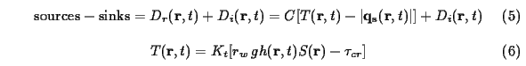
where T is the sediment transport capacity [kg/(ms)],
D_r is the rill erosion or deposition rate,
D_i is the interrill contribution [kg/(m.m.s)],
C is the first-order reaction coefficient dependent
on soil and cover [1/m],
r_w is the mass density of water [kg/m.m.m],
S(r)=grad z(r) is the slope [m/m],
z(r) is the elevation [m],
Kt is the transport capacity coefficient,
g=9.81 is gravitational acceleration [m/s.s.s].
We assume that the critical sheer stress tau_c is
negligibly small.
Rill detachment and deposition are
proportional to the difference between transport capacity and sediment load
(eq. 5). This relationship defining the interaction
between sediment load and transport capacity (Foster and Meyer, 1972) is
based on a stream power concept (Haan 1994) and can be expressed as:

where D_c=C.T=K_d.r_w.g.h.S is the detachment capacity
and K_d is the detachment capacity coefficient (rill erodibility).
We solve the continuity equation in 2D form
for steady state water flux with small diffusive term with
amplitude d,
rewritten in the operator form as:
where rho=r_s.c.h.
The interpretation of the equation (8) is clear: the first term is the diffusion
(which in our case is very small and represents the smoothing
component of the soil transport),
the second term is the drift driven by the water velocity v(r)
and the third term is the 'potential' which is dependent on the velocity
magnitude: the larger the velocity, the smaller the concentration of sediment.
Net erosion and deposition is then estimated as a divergence of sediment flux. Further details about this approach and comparisons with previous estimations of erosion/deposition by the directional derivative (Mitasova et al. 1995, Wilson and Moore 1992) will be given in Mitas and Mitasova, (in prep.).
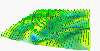
The equation (8) is solved analogically as the equation for water flux using a stochastic method (Mitas and Mitasova, in prep.), illustrated by Movie 1.:
In the erosion model the influence of soil and cover is represented by the following basic parameters: Mannings n , detachment rate coefficient (erodibility) Kd, and sediment transport coefficient Kt. These coefficients are functions of soil and cover properties such as soil texture, canopy, roots, management practices etc., and their estimation and development of various adjustment factors is described in WEPP (Flanagan and Nearing 1995). Constants for estimation of detachment and sediment transport capacity are still under development and detailed discussion of these parameters is beyond the scope of this paper. However, we will use the following examples to elucidate the role of these parameters in modeling spatial distribution of areas with erosion or deposition.
The most important parameter controlling the borderline between the erosion and deposition is the first-order reaction coefficient C related to the ratio of detachment capacity and sediment transport capacity. In the first example, we simulate the situation when the study area has constant transport capacity coefficient Kt but detachment capacity coefficient Kd increases, so that the ratio C increases from 0.0005 to 100 (Movie 2).
For small values of C (e.g., clay with very low fall velocities and low detachment capacity) water has the power to carry almost all detached sediment into the stream. For values C>1 ( e.g., sandy soils with relatively high fall velocities which detach easily), the sediment flux quickly reaches the sediment transport capacity and deposition occurs relatively high in the hillslope. This is the case of transport limited erosion/deposition modeled by a simplified approach described e.g., by Mitasova et al. 1996 and Moore and Wilson 1992. For both cases the magnitude of sediment flux in the stream remains the same while the distribution of erosion and deposition over the landscape changes significantly. This simulation is a good example which shows that calibrating the erosion model using only the observed values of sediment flux at an outlet does not guarantee correct predictions of erosion/deposition on the complex hillslopes within the watershed.
Change in Kt while Kd is constant also changes the spatial distribution of erosion/deposition, however there is a big difference in the amount of sediment delivered to streams. For Kt<<Kd and C>>1 most of the detached material deposits before it enters the stream, for Kt>>Kd and C<<1, there is only a very small deposition and most of the detached material is delivered into streams (Movie 3). This example illustrates how the potential changes in soil properties and cover which increase transport capacity can trigger severe erosion.
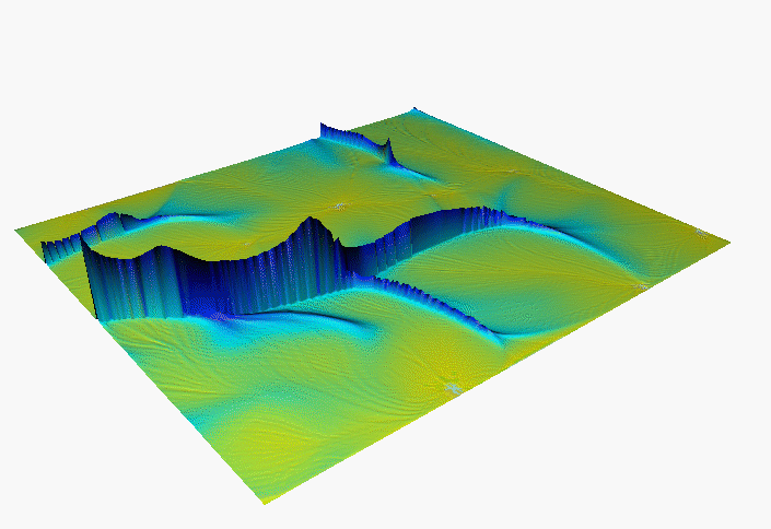
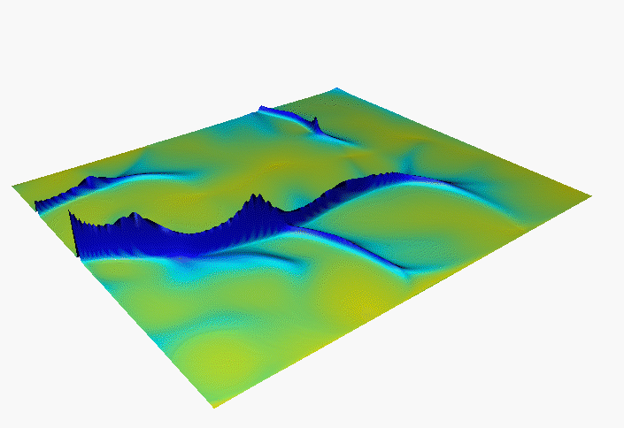
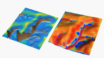
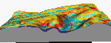
If C=const. and Kt, Kd change with the same rate, the spatial distribution of erosion/deposition is the same, and only its magnitude changes (Figure 2.)
 a, b
a, b
Figure 2. Change in the magnitude of erosion/deposition with C=1 and increase in both Kt and Kd; a)n=0.1, Kd=Kt=0.0003 (grass on sandy soil); b)n=0.05, Kd=Kt=0.03 (bare sandy soil). Surface topography represents the sediment flux, color is the erosion/deposition.
It is important to note that the parameters Kt and Kd which are dependent on the soil and cover properties are interrelated and the change in one parameter is usually accompanied with the change in the second parameter. As we have demonstrated, it is their ratio, which plays important role in the spatial distribution of erosion and deposition. With better understanding of the physical basis of these parameters the analysis outlined above can be used for identification of those soil and cover properties which can be targeted for the most effective erosion prevention.
Erosion process is highly dynamic and its temporal variability can be modeled at various time scales from minutes (event based models such as ANSWERS or AGNPS), days (WEPP), to geological time (Moglen and Brass 1994). For land use management applications we adapt the concept used in WEPP and we simulate erosion under steady state flow for variable climatic, soil and cover parameters as they change during the year.
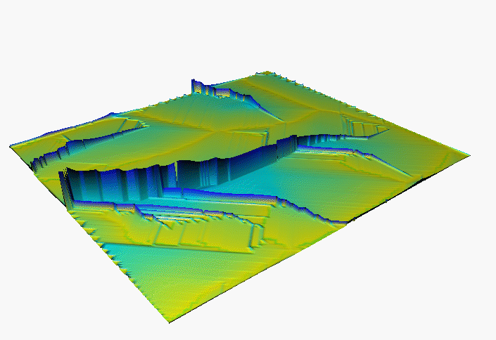
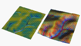
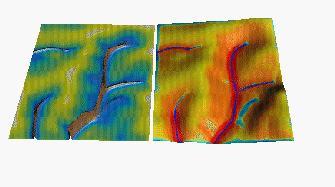
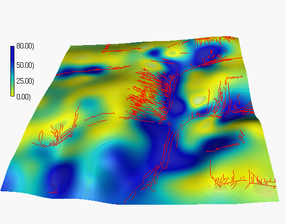
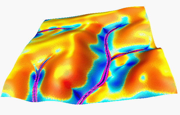
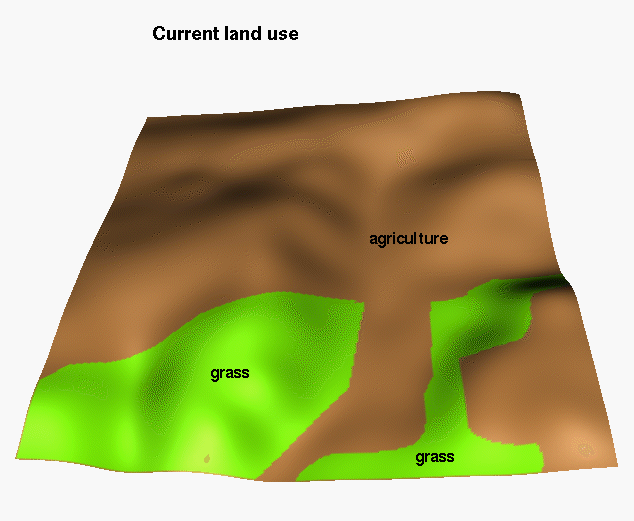
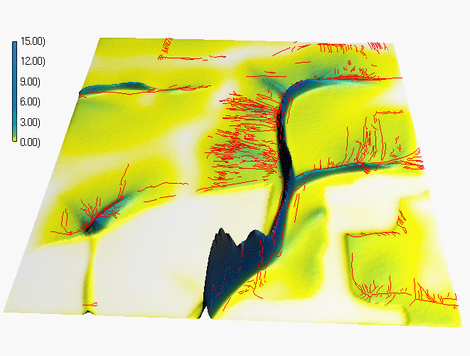
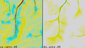
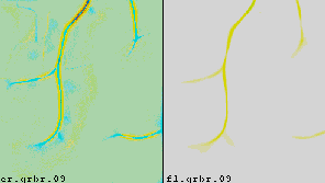
To evaluate the predictive capabilities of the proposed model, we have used elevation, soil and land use data from an experimental farm of the Technical University in Munchen, Germany (courtesy Dr. Karl Auerswald). We simulated sediment flux and erosion/deposition for the current land use with various cover and rainfall conditions. Comparison of the results with the observed spatial distribution of colluvial deposits (Figure 3) and with the pattern of linear erosion after an extreme storm (Figures 3, 4) indicates, that for this area with mostly sandy soils, the terrain controls the long term spatial pattern of deposition reflected in colluvial deposits observed in mostly concave areas (Figure 3a, Movie 4). Land cover seems to have more significant impact on the magnitude of erosion and short term linear erosion features (Figure 4).
 a
a
 b
b
 a
a
 b
b
 c
c
We have also simulated the changes in erosion/deposition during a year
due to the changes in rainfall and land cover, illustrated by Movie 5. and
Figure 5.
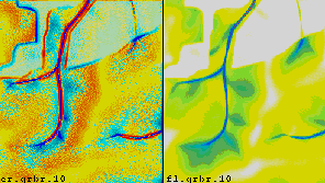
The highest risk of erosion was predicted in October, when there is minimum cover and enough rainfall to produce significant runoff. Although May had the most intense storm, the erosion was lower due to the good cover provided by both the grass area and the agricultural area with winter wheat.
Human activity changes character or properties of landscape
components (e.g. cover) which can be represented
as an appropriate change in the corresponding field.
These changes influence the natural phenomena
through various interactions which can be described
by the governing master equations.
Well-defined and quantified impact of human actions on nature
enable researchers to formulate
objectives or costs in order to either predict the future development or,
more importantly, to achieve a desired sustainable development.
The desired objectives can include, e.g.,
maximization of land use for production
or military training with minimized
impact on environment, or prevention of unacceptable changes
in environment in the given time horizon with minized costs
(Johnston and Hopkins 1994).
Because of the extremely complex nature of the problem,
the optimization tasks are often out of the scope of ordinary
techniques as they involve
multivariate fields (possibly evolving in time) and also because of the
special type of human action (like instantaneous point sources
such as contamination which spreads out in the time horizon of a few
years or clear cut of a forest with consequent erosion).
Therefore this problem requires a formulation
of general methods which can deal
with complicated types of "configuration or state spaces".
For our case we can define
the state space as a set of fields (i.e., a particular
set of multivariate
functions) which describe components of the studied phenomenon.
Available information and models such as initial fields values,
are provided by a GIS and are used as inputs into the master
equations and their solvers.
In addition, we need to express the objective
(cost) functional which is to be minimized within given constraints.
The constraints can be formulated in the form
of ``external'' fixed influences (e.g. part of land cover which cannot
be changed), thresholds on evolving fields (e.g. erosion beyond
certain level is unacceptable) and so forth.
The general form of the cost functional can be given as:

where I is the cost functional, z_i are the
input spatio-temporal fields, F is a function which
determines the cost for a particular set of z_i
(point in the state space).
In general, a minimization of (10) can be a very
complex task.
In order to carry out the minimization of the functional (10) we
have to define the following:
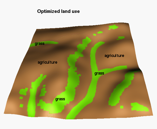
A simple example of using GIS and the erosion model to optimize
land use by finding a more effective spatial distribution
of protective grass cover while keeping the ratio between the
agricultural area and area protected by grass constant
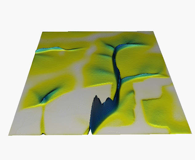
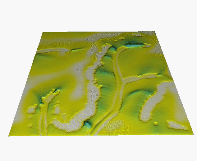
is illustrated in Figures 6 and 7. Under the current land use (Figure 6a),
there is still a significant amount of sediment delivered
to the stream (Figure 6b) with strong potential of creating rills and
gullies (Figure 6c, dark red) which is in agreement with observations
of big storm effects, presented in Figure 4.
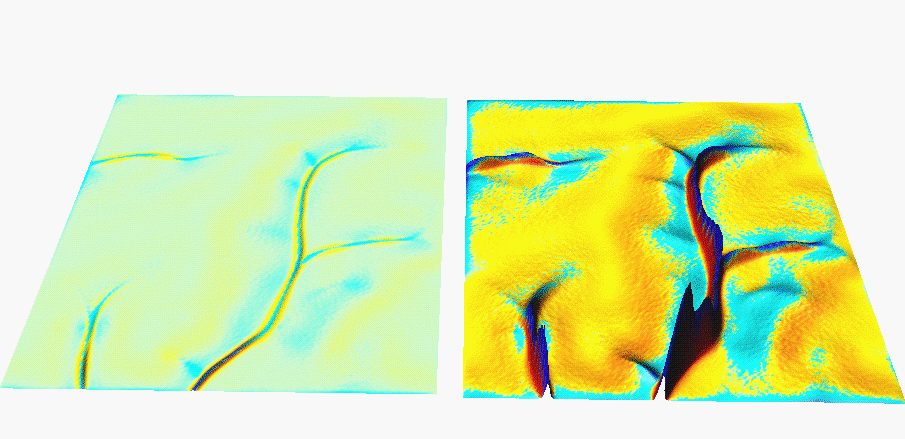
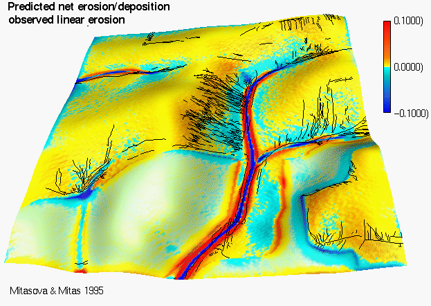
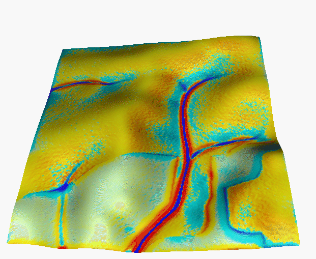
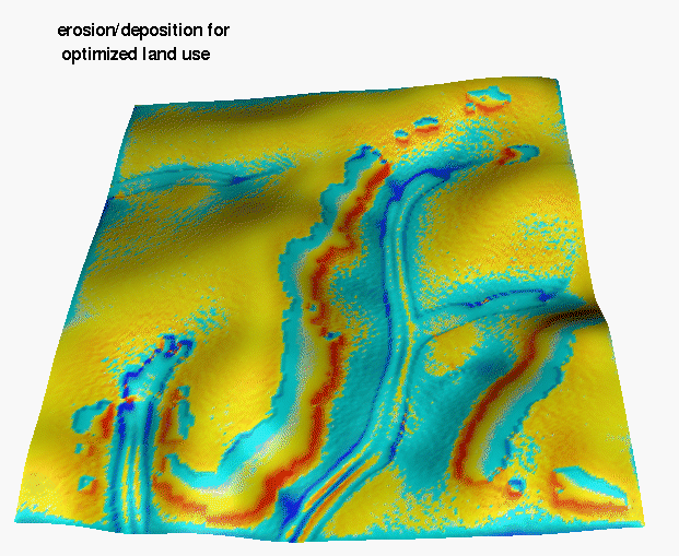
Redesigning the land use so that the protective grass cover
is located in the highest erosion risk areas (Figure 7a)
can dramatically reduce soil loss and sediment delivery to
the streams (Figure 7b,c). The crest in sediment flux in
areas with observed gullies disappears and is replaced by
light deposition caused by the decrease in water velocity in the grass strip
(Figure 7c).
a
 b
b
 c
c
 a
a
 b
b
 c
c
We have presented an approach to modeling of landscape processes in an advanced GIS environment which is based on the following developments :
Important computational components of our approach such as interpolation tool, water flux solver, sediment flux solver, scenario optimizer (under current development) are built as functional units with well-defined input, output and controls. Therefore these units can be used either as separate tools or within open GIS frameworks such as GRASS depending on the computational environments and size of tasks.
Using the presented application as an example, we believe that the GIS in future can become not only a powerful tool for providing and analyzing spatial information, but by extending its capabilities as a simulation and optimization tool, it can allow its users to find unexpected solutions of land management problems leading to practices which can be more effective at lower cost than the currently known conservation approaches.
Berry, M.W, Flamm R. O., Hazen B. C., MacIntyre, R.L.(1995).
The Land-Use Change Analysis System (LUCAS) for Evaluating Landscape
Management Decisions. IEEE Comp. Science and Engn., (in press).
http://www.cs.utk.edu/~lucas/
Brown, W.M. and Shapiro, M. (1995).
DateTime Library.
http://softail.cecer.army.mil/~brown/doc/dt_pman.html
Brown, W.M. and Astley M. (1995).
NVIZ tutorial.
http://www.cecer.army.mil/grass/viz/nviz.tut.html
Cox, S. (1994).
Toward a Fission Track Tectonic Image of Australia: Model based
interpolation in the Snowy Mountains using a GIS.
http://www.ned.dem.csiro.au/AGCRC/papers/snowys/12agc.cox.html
Engel, B. (1995). Hydrology Models in GRASS. http://soils.ecn.purdue.edu:80/~aggrass/models/hydrology.html
Flanagan, D.C. and Nearing, M. A. (1995).
USDA-Water Erosion
Prediction Project
(WEPP), NSERL report No. 10
National Soil Erosion Lab., USDA ARS, Laffayette, IN
Foster, G.R. and Meyer, L.D. (1972). A closed-form erosion equation for upland areas. Sedimentation: Symposium to Honor Prof. H.A.Einstein (Shen, ed.), Chap. 12, pp.12-1-12.19. ColoradoState University, Ft. Collins, CO
Garrote, L. and Bras, R.L. (1993). Real-time modeling of river basin response using radar-generated rainfall maps and a distributed hydrologic database. Report No. 337. MIT, Cambridge, Massachusets.
Govindaraju, R.S. and Kavvas, M.L. (1991). Modeling the erosion process over steep slopes: approximate analytical solutions. Journal of Hydrology 127, 279-305.
Haan, C.T., Barfield, B.J., Hayes, J.C. (1994). Design Hydrology and Sedimentology for Small Catchments. Academic Press.
GRASS4.1 Reference Manual (1993). U.S.Army Corps of Engineers, Construction Engineering Research Laboratories, Champaign, Illinois, 422-425.
GRASS4.2 new libraries.
http://www.cecer.army.mil/grass/grass42_new_api.html
Hargrove (1995). Clinch River Environmental Restoration Program. http://www.esd.ornl.gov/programs/CRERP/
Johnston, D.M. and Hopkins, L.D,
TRAINER:
a System for training
requirements assessment and Integration with environmental resources.
http://ice.gis.uiuc.edu/trainer_html/trainer.html
Leavesley, G.H., Restrepo, P.J., Stannard, L.G., Frankoski, L.A.
and Sautins, A.M. (1996).
MMS: A Modeling Framework for Multidisciplinary Research and Operational
Applications. GIS and Environmental Modeling: Progress and Research
Issues (Goodchild, M.F., Steyaert, L.T. and Parks, B.O., eds.),
GIS World, Inc.,pp.155-158.
http://www.terra.colostate.edu/projects/mms.html
Maidment, D.R. (1996). Environmental modeling within GIS.
GIS and Environmental Modeling: Progress and Research
Issues (Goodchild, M.F., Steyaert, L.T. and Parks, B.O., eds.),
GIS World, Inc.,pp.315-324.
McCauley (1995).
GRASS 4.2 Sites Format and API.
http://www.cecer.army.mil/grass/sites-api/index.html
H. Mitasova, L. Mitas, W.M. Brown, D.P. Gerdes, I. Kosinovsky and T. Baker (1995). Modeling spatially and temporally distributed phenomena: new methods and tools for GRASS GIS, International Journal of Geographical Information Systems, 9, 433-446.
Mitasova, H., Hofierka, J., Zlocha, M., and Iverson, R.L. (1996) Modeling topographic potential for erosion and deposition using GIS. Int. Journal of Geographical Information Systems (in press).
Moglen G.E. and Bras R.L. (1994). Simulation of observed topography using a physically-based basin evolution model. Report No. 340. MIT.
Moore, I.D., Turner, A.K., Wilson, J.P., Jensen, S.K., Band, L.E., (1992). GIS and Land-Surface-Subsurface Modeling. Geographic Information Systems and Environmental Modeling, (Goodchild, M.F., Parks, B., Steyaert, L.T., eds.), Oxford University Press, New York, pp. 196-230.
Moore, I.D., and Wilson, J.P., (1992). Length-slope factors for the Revised Universal Soil Loss Equation: Simplified method of estimation. Journal of Soil and Water Conservation, 423-428.
Mitas and Mitasova (1996). Distributed erosion/deposition simulations, in preparation.
Rewerts C.C. and Engel B.A., (1991). ANSWERS on GRASS: Integrating a watershed simulation with a GIS. ASAE Paper No.91-2621. American Society of Agricultural Engineers, St.Joseph, Missouri, 1-8.
Vieux, B.E., Farajalla, N.S. and Gaur N. (1996). Integrated GIS and distributed
storm water runoff modeling.
GIS and Environmental Modeling: Progress and Research
Issues (Goodchild, M.F., Steyaert, L.T. and Parks, B.O., eds.),
GIS World, Inc.,pp.199-205.
Saghafian, B., (1996). Implementation of a Distributed Hydrologic Model within
GRASS.
GIS and Environmental Modeling: Progress and Research
Issues (Goodchild, M.F., Steyaert, L.T. and Parks, B.O., eds.),
GIS World, Inc., pp.205-208.
Waupotitsch and Shapiro (1995). Floating-Point / NULL Values in GRASS Raster Maps. http://softail.cecer.army.mil/~olga/fpnv.html
Helena Mitasova
Geographic Modeling and Systems Laboratory
Department of Geography
220 Davenport Hall
University of Illinois at U-C
Urbana, IL 61801
helena@gis.uiuc.edu
Telephone: (217) 333-4735
FAX: (217) 244-1785
William M. Brown
Geographic Modeling and Systems Laboratory
Department of Geography
220 Davenport Hall
University of Illinois at U-C
Urbana, IL 61801
brown@gis.uiuc.edu
Telephone: (217) 333-5077
FAX: (217) 244-1785
Mark Astley
Geographic Modeling and Systems Laboratory
Department of Geography
220 Davenport Hall
University of Illinois at U-C
Urbana, IL 61801
m-astle@uiuc.edu
Telephone: (217) 333-4764
FAX: (217) 244-1785
 GMSL Modeling & Visualization