


February - November 1997
September - December 1997
Prepared by:
Geographic Modeling and Systems Laboratory, University of Illinois at Urbana-Champaign, Urbana, Illinois
H. Mitasova, L. Mitas, W.M. Brown, D. Johnston
Prepared for:
U.S.Army Construction Engineering Research Laboratories
S. Warren
Urbana, November 1997, http://www2.gis.uiuc.edu:2280/modviz/reports/cerl97/rep97.html
1. Introduction..........................................................................................................................3
2.
Methods................................................................................................................................4
2.1 Unit stream power based erosion/deposition
model (USPED)....................................4
2.2 Process-based simulation of water erosion (SIMWE).................................................7
2.2.1 Impact of spatially uniform parameters in complex terrain................................7
2.2.2 Transport and detachment capacity equations (V).............................................10
2.2.3 Impact of spatially variable land cover (V)........................................................11
2.2.4 Impact of temporal variability in land cover......................................................12
2.2.5 Simulation of impact of terrain structures..........................................................14
3. GIS tools (V)......................................................................................................................14
4. Applications to military installations................................................................................16
4.1 Ft. Irwin........................................................................................................................16
4.2 Ft. McCoy (V)..............................................................................................................22
5. Conclusion, future directions.............................................................................................25
6. References...........................................................................................................................26
7. Full size figures (for printed version)................................................................................30
Note: Chapters (V) describe work performed for the PART V contract, the rest is for the PART IV contract.
To fulfill the need for better understanding of spatial and temporal distributions of phenomena resulting from landscape processes, empirical models based on lumped, averaged parameters are being replaced by process-based distributed models supported by Geographic Information Systems (GIS) (Moore et al. 1993, Maidment 1996, Engel 1995, Vieux et al. 1996, Saghafian 1996). Over the last few years there has been a remarkable progress in development of tools for studies of hydrological processes represented, e.g., by the CASC2d model (Saghafian 1996) and others (Garrote and Brass 1995, Vieux 1996). While these developments enhanced the capabilities to estimate overland flow in complex terrain, the development of distributed, process-based simulations of erosion, sediment transport and deposition at similar levels of realism has been slower, due to the enormous complexity of processes involved. Most of the current process-based erosion models can be roughly divided into three main groups:
a) field scale models developed for soil conservation (e.g., WEPP) which are based on a 1D flow over hillslope segments (Foster et al. 1995). They incorporate the impact of soil, cover and management practices with a great detail, however, the description of topography is very simplified. Data preparation for larger and complex fields can be time consuming and results are given only for profiles or as statistical averages or integrals for entire hillslopes or small watersheds.
b) watershed scale models designed for water quality applications focus on predicting sediment loads and concentrations of chemicals delivered to and transported through streams using channel routing (e.g., Arnold et al. 1993, Srinivasan and Arnold 1994, Rewerts and Engel 1991). The overland flow related processes are modeled using sets of homogeneous hillslope segments or subwatersheds with lumped parameters.
c) landscape scale models simulating the landscape evolution by geomorphological processes which describe the changes in topography at the temporal scales from hundreds to thousands of years (e.g., Kirkby 1986, Willgoose et al. 1991, Kramer and Marder 1992, Howard 1994).
Although this categorization is hardly exhaustive and there are several models which combine more than one of the above given concepts, a number of issues important for effective erosion prevention at a landscape scale remain unresolved. Many existing methods require large number of empirical inputs, important effects of terrain shape are not taken fully into account, numerical methods used for the model implementations exhibit instabilities when used at high resolutions, and detailed spatially variable outputs are limited. Combination of these factors often make applications of traditional models either laborious or simply not practical, especially for large areas. Some of the key unsolved modeling issues which restrict the use of the current models to increase our knowledge about spatio-temporal aspects of erosion processes and limit their application to effective erosion prevention for large, complex areas can be identified as follows:
a) high resolution treatment of complex terrain, land use and soils in a fully 2D/3D distributed manner,
b) description of processes at a fundamental level with minimal number of empirical inputs and availability of robust and efficient process solvers to minimize tedious manual modifications of data,
c) integration of models at different spatial and temporal scales,
d) validation of both spatial and quantitative aspects model of predictions. While the capabilities to qualitatively predict some spatial aspects of erosion and deposition improved (Mitas and Mitasova 1998a), the quantitative estimates are still very problematic (e.g., Bjorneberg et al. 1997 reports soil loss predictions from WEPP of 200 kg/m when measured soil loss was less than 5 kg/m, Johnson et al., 1997 reports several results from estimation of sediment yield by CASC2D-SED with 100-400% differences between the computed and observed yields). Closer correspondence between experiments and models is needed.
e) low quality of available digital elevation models which require sophisticated re-processing or manual modifications to make them usable for process modeling.
f) development of soil and cover parameters for process-based models requires an ongoing extensive experimental work, while the relationships between these parameters is not very well understood.
g) providing numerical, graphical and cartographic outputs in a form which enables easy spatial analysis and supports decision-making process.
It is clear that resolving these complex issues will require considerable time and effort of many research teams, therefore in this project we focus on a selected subset of the problems, especially those which we believe are relevant to erosion modeling at military installations. In this report, we focus on the most recent enhancements of our models, we elucidate the role of input parameters and illustrate the a use of simulations for land use management. In applications part we demonstrate and discuss the technical issues related to routine applications of erosion simulations to military installations.
The methods and GIS tools which we have developed to support modeling of erosion, sediment transport and deposition in complex terrain are described in the previous reports (Mitasova et al. 1995, 1996ab) and publications (Mitasova and Mitas 1993, Mitas and Hofierka 1993, Mitasova et al. 1995, Mitasova et al. 1996, Mitas and Mitasova 1997, Mitas et al. 1997, Mitas and Mitasova 1998a,b)). In this report we briefly recall the principles of these methods and focus on the most recent developments.
The original version of the USPED model is described in Mitasova et al. (1996ab), therefore here we only briefly recall its principles. USPED is a simple model which predicts the spatial distribution of erosion and deposition rates for a steady state overland flow with uniform rainfall excess conditions for transport capacity limited case of erosion process. Sediment flow rate is approximated by sediment transport capacity T(r), r=(x,y) which is computed as a power function of slope ß(r), upslope area A(r) and transportability coefficient K(r) dependent on soil and cover. Net erosion and deposition is computed as a change in sediment flow rate. In this report we compare the original formulation of USPED (Mitasova et al 1996a) with an improved version derived as a special case of the SIMWE model (Mitas and Mitasova 1998a).
Improved impact of topography. Within the original USPED the water and sediment flow is modeled as 1D flow along a flow line generated over 3D terrain. The net erosion/deposition rate is computed as a change in the sediment flow rate along the flow line, approximated by a directional derivative of the sediment flow rate. For this univariate case, the net erosion/deposition rate D(r) is
D(r) = dT(r)/ds = K(r) {[ grad h(r) . s(r) ] sin ß(r) - h(r) kp(r)} (1)
where r=(x,y), s(r) is the unit vector in the steepest slope direction, h(r) is the water depth estimated from the upslope area A(r), kp(r) is the profile curvature (terrain curvature in the direction of the minus gradient, i.e., the direction of the steepest slope). This 1D flow-based formulation includes the impact of water flow, slope and profile curvature, however, the impact of tangential curvature is incorporated only through the water flow term. The predicted pattern is in a good agreement with observations except for heads of valleys where it predicts only erosion while the soil maps and field experiments indicate that both deposition and erosion is observed, and for shoulders where it does not predict commonly reported local maximum in erosion rates (Martz 1987, 1991, Sutherland 1991, Quinne et al. 1994).
Within the 2D flow formulation, which was derived as a special case of the more general model SIMWE (Mitas and Mitasova 1998a) we represent the water an sediment flow as a bivariate vector field q(r)=q(x,y), qs(r)=qs(x,y). Then, the net erosion/deposition rate is estimated as a divergence of the sediment flow. If we assume uniform rainfall, soil and cover conditions, and a transport capacity limiting case with sediment flow close to sediment transport capacity, the net erosion/deposition can be written as (see Appendix in Mitas and Mitasova 1998a):
D(r) = div qs(r) = K(r) { [grad h(r)] . s(r) sin ß(r) - h(r) [kp(r) + kt(r)] } (2)
where kt(r) is the tangential curvature (curvature in the direction perpendicular to the gradient, i.e., the direction tangential to a contourline projected to the normal plane). Topographic parameters s(r), kp(r), kt(r) are computed from the first and second order derivatives of terrain surface approximated by the regularized spline with tension (RST) (Mitasova and Mitas, 1993; Mitasova and Hofierka, 1993; Krcho 1991). According to (2), the spatial distribution of erosion/deposition is controlled by the change in the overland flow depth (first term) and by the local geometry of terrain (second term), including both profile and tangential curvatures. The equation (2) thus demonstrates that the local acceleration of flow in both the gradient and tangential directions (related to the profile and tangential curvatures) play equally important roles in spatial distribution of erosion/deposition. The impact of the tangential curvature kt(r) is therefore twofold. First, kt(r) influences the water depth h(r) through its control of water flow convergence/divergence, with tangential concavity leading to rapid increase in water depth and an increase in the potential for erosion (first term in (2)). Second, kt(r) causes a local change in sediment flow velocity which for tangential concavity has an opposite effect (reduction in sediment transport), creating thus potential for deposition. The interplay between the magnitude of water flow change and both terrain curvatures reflected in the equation (2) therefore determines whether erosion or deposition will occur.
When the results of the 1D flow (Figure 1c) and the 2D flow (Figure 1b) models are compared with the observed pattern of colluvial deposits (Figure 1a), it is clear, that equation (1) fails to predict deposition observed in areas where profile curvature is close to zero but there is a significant tangential concavity (areas A and B in Figures 1abc). It also underestimates erosion in areas with tangential convexity (shoulders) . The prediction by the 2D flow model in these areas is in significantly better agreement with the observed pattern of deposition. The 1D flow model underestimates the overall extent of deposition as only a 18% of the total area, while the 2D flow model, without taking into account the spatial variability in surface cover, predicts deposition at 26% of the total area. Colluvial deposits thicker than 10cm, indicating long term deposition, were observed in 40% of the sampling sites. The sedimentation area observed on a steep hillslope covered by grass, which contributes to the spatial extent of deposition (Figure 1a) cannot be predicted by using only the elevation data and the incorporation of spatially variable cover is necessary.

Figure 1. Full
incorporation of topography for transport capacity limited erosion : a)
observed depths of colluvial deposits, b) erosion and deposition
pattern from 2D flow formulation of USPED, c) erosion and deposition
pattern from 1D flow formulation of USPED, d) water flow term, e)
profile curvature term, f) tangential curvature term.
The 2D flow equation (2) also provides a sound theoretical explanation for the results of field experiments reported by several authors, e.g., Busacca et al., (1993) and Sutherland, (1991); where `the highest erosion was observed on divergent shoulder elements and deposition on convergent footslope elements', as well as by Heimsath et al., (1997), or Quine et al. (1994) observing `maximum soil loss from the slope convexities and maximum gain in both the slope concavities and the main thalwegs'.
Computer implementation of the more complete USPED equation (2) is rather simple, using the tools already developed for this project. Water depth h = A i n / sqrt (sin ß)**0.6 is estimated from upslope contributing area A computed from a DEM using r.flow program (Mitasova et al. 1996b), while topographic parameters (slope ß, aspect and curvatures) are computed by interpolation program s.surf.rst (Mitasova et al. 1995b), r.resamp.rst (Mitasova et al. 1996b) or by enhanced r.slope.aspect (Appendix) . The i is rainfall excess and n is Mannings roughness coefficient. The equation for h and the equation (2) for net erosion/deposition D(r) are then computed using r.mapcalc.
Influence of rainfall, soil and cover properties. Soil and cover parameters similar to those used in USLE or WEPP were not developed for the USPED model, as no systematic experimental work was performed. However, it was suggested (Moore and Wilson 1992) that under certain conditions, there is a relation between the USPED concept and USLE. It is therefore possible to combine the model with the USLE/RUSLE factors to predict the relative impact of land use change on erosion/deposition pattern assuming the conditions valid for USPED hold. This approach was used e.g., for the Camp Shelby study (Mitasova et al., 1996b). Caution should be used when interpreting the results because the USLE parameters were developed for simple plane fields and to obtain accurate predictions for complex terrain conditions they need to be re-calibrated ( Foster 1990, Mitasova et al 1997 reply).
The SIMWE model is described in the previous report (Mitasova et al. 1996c) and in Mitas and Mitasova (1998a), therefore we present here only a brief concept and focus on the role of the parameters. SIMWE is a landscape scale, bivariate model of erosion and deposition by overland flow designed for spatially complex terrain, soil and cover conditions. The underlying continuity equations are solved by Green's function Monte Carlo method, to provide robustness necessary for spatially variable conditions and high resolutions. We use the experimental farm data described in Mitasova et al. (1995b, 1996b) and by (Auerswald et al. 1996), to explain the role of the parameters and to elucidate how natural phenomena and properties influence the erosion process.
Meyer and Wischmeier (1969) presented an erosion model based on principles later formulated as a closed form erosion equation by Foster and Meyer (1972) and used in the WEPP, CREAMS and numerous other models (Hong and Mostaghimi 1995, Haan et al. 1994) including SIMWE. They formulated the model for a 1D complex profile and analyzed its behavior for various combination of parameters, elucidating thus the impact of different terrain, rainfall, soil and cover properties on distribution of erosion and deposition rates along a profile. The following examples represent a generalization of this analysis to terrain represented by bivariate (2D) function in a 3D space.
In this analysis the baseline situation for all examples is 36mm/hour rainfall intensity, full saturation, (therefore rainfall intensity = rainfall excess rate), rough surface (e.g., dense grass with Mannings n = 0.1), sandy type of soil (negligible critical shear stress, with low detachability (erodibility) and low transportability due to the dense cover and larger particle size: Kt = Kd = 0.0003). The following examples illustrate how the magnitude and pattern of erosion/deposition rates changes due to the change in one of the parameters.
Rainfall excess is estimated as rainfall intensity - infiltration rate where infiltration rate can be estimated from a separate module or using r.mapcalc based on the soil data. Rainfall excess influences the magnitude of erosion/deposition rates, with increasing rainfall excess both the erosion and deposition rates increase, however the spatial pattern of erosion and deposition does not change (Figure 2).
Figure 2. Impact of increasing rainfall excess a) r = 36 mm/h, b) r = 72 mm/h, c) r = 144 mm/h.
Surface roughness, represented in our case by the Manning's
coefficient, influences water and sediment flow velocities. Surface
roughness parameter depends on vegetation cover as well as the soil
surface and its values for variety of situations have been derived from
experiments and are available from literature and the WEPP users
manual. The change in surface roughness changes the erosion and
deposition pattern. In our example, the extent of deposition for smooth
surfaces n=0.01 is predicted only for locations with strong
profile and tangential concavity covering about 14% of the total area
while for rough surfaces with n=0.1 the extent of deposition is
closer to the transport capacity limiting case, covering more than 24%
of total area (Figure 3).
Figure 3. Impact of surface roughness a) n=0.01 (smooth surface), b) n=0.10 (rough surface).
Critical shear stress represents the soils resistance to the
shearing forces of water flow. It depends on soil and cover properties
and the values are available e.g., from the WEPP manual (Flanagan and
Nearing, 1995). If shear stress at the given location is lower than the
critical shear stress, no soil is detached. This parameter therefore
has an impact on erosion/deposition pattern. Its high value reduces the spatial
extent of erosion, on the other hand, it can also increase the
magnitude of erosion rates on steeper hillslopes and in areas with
concentrated flow due to the fact that clean water has higher potential
to transport the sediment (Figure 4).
Figure 4. Impact of uniform critical shear stress a) 1.0, b)3.0, c) 7.0.
Erodibility (detachment capacity coefficient) is a measure of
soil susceptibility to detachment by water flow (Flanagan and Nearing,
1995). It is often defined as the increase in soil detachment per unit
increase in shear stress of clear water flow. Change in erodibility
factor while keeping the other parameters constant changes the ratio
between transport capacity and detachment capacity . This leads to the
change in the character of erosion process from detachment capacity
limited for erodibility significantly lower than transportability
to transport capacity limited case when erodibility is
greater than transportability. Therefore, as shown in the animation
(Figure 5), change in erodibility will change the spatial pattern of
erosion and deposition, however the impact on the magnitude of the
sediment load in stream is small. This example is a good illustration
of the fact that measuring sediment load in the watershed outlet does
not provide enough information for understanding the erosion processes
on watershed's hillslopes and quite different processes can result in
the same sediment concentration levels. This makes the use of instream
sediment concentrations as a measure reflecting the impact of erosion
protection measurers needed for land use management problematic.
Figure 5. (animation) Impact of change in soil erodibility Kd=(0.0001,0.1), Kt=0.001 .
Transportability or transport capacity coefficient is a measure of soil capability to be transported by water flow. It depends on soil properties but can be also influenced by vegetation. This coefficient is not directly measured and provided in the WEPP, rather it is estimated indirectly, which is making the proper determination of this parameter problematic. However, the parameter can be derived at least for some types of soils using the published values of first order reaction coefficient or using the procedure suggested by Finkner et al. (1989). Our simulations show that this parameter has a profound impact on the erosion process as it influences both spatial distribution and magnitude of sediment flow and erosion/deposition rates. Recently, the importance of transport capacity for overland flow erosion processes is being fully recognized and more experimental and theoretical work is being performed (Guy et al. 1991, Govers 1991, Nearing et al. 1997). We further discuss this issue in a separate chapter. The following animation illustrates how the change in transportability changes the erosion regime from detachment capacity limited to transport capacity limited while also reducing the magnitude of erosion rates.
Figure 6. (animation) Impact of change in soil transportability: Kd=0.001, Kt=(0.0001,0.1)
It is important to note that the parameters do not act independently, they are interrelated and it is this interaction which controls the pattern and magnitude of erosion. For example, the growth of vegetation reduces both Kd, Kt and 1/n and the resulting erosion/deposition pattern depends on the interaction between the rates of this change. If both Kd and Kt change at the same rate, the spatial distribution of erosion/deposition stays the same and only the magnitude of rates changes. If vegetation growth reduces Kd faster than Kt, the erosion/deposition pattern will change from transport capacity limited towards detachment limited. The interrelation between the parameters is an open research question and there is a lack of systematic experimental and theoretical/modeling work in this area.
The presented analysis shows that for the uniform soil and cover there is a basic pattern of erosion and deposition in complex terrain which does not change significantly even if rainfall, soil and cover changes. High erosion risk areas are located on upper convex parts of hillslopes and in hollows and centers of valleys with concentrated flow. Deposition occurres in concave valleys and concave lower parts of hillslopes. With changing soil and cover conditions the line of starting deposition can move up- or down-slope, potentially influencing the sediment loads in streams. The analysis demonstrates that besides the obvious fact that the worst situation occurs for large events with high rainfall intensity when the soil surface is rather smooth (e.g. without a protective vegetation cover), sediment loads can be very high even for smaller events if soil is highly transportable. Change in the soil and cover from a uniform to spatially variable distribution has a great impact on the basic pattern of erosion/deposition (as we show later). Depending on the location this spatial variability can positively or negatively influence the overall soil loss as well as the sediment loads in streams.
Our previous simulations (Mitas and Mitasova 1998) as well as several recent publications ( Govers 1991, Guy et al. 1991, Nearing et al. 1997) indicated that the transport capacity equation used in the WEPP model is probably not general enough for use in complex terrain conditions. Similar suggestions were made also about the detachment equation used in WEPP (Bjorneberg et al. 1997). For example, we were not able to reproduce completely the extent of areas with observed deposition. To address this issue we have attempted to study the sediment transport capacity relations as the key influencing quantity in our applications. We have tested both the power law shear stress relations (Julien and Simon 1985) with different power exponents and the new stream power based relation suggested by Nearing and co-workers (1997).
Julien and Simon (1985) analyzed the existing sediment transport equations and presented an equation in a general form:
qs = p q m sin ß n i d (1- t0 / t) e (3)
where qs is the sediment flux, q is the water flux, ß is the slope angle, i is the rainfall intensity, t0, t are the critical shear stress and shear stress respectively, and p, m, n, d, e are experimental or physically based coefficients. The WEPP uses this equation with m=n=1.5. We have tested it for values of m=0.6-2.0. Willgoose (1989) has shown that the parameter m depends on the type of flow and channel geometry which indicates that in complex terrain and cover conditions this coefficient should be spatially variable depending on the type of flow in a particular area. Higher values of m lead to greater impact of water flow on erosion pattern, while for the lower values of m, terrain has more profound impact (see Figure 30 in applications).
For modeling erosion in a rill Nearing et al. (1997) presented an improved fit to several sets of experimental data by relating sediment load qs to stream power o:
log qs = A + {B exp (C + D log o) / [1 + exp (C + D log o)]} (4)
with the constants A = -34.47, B = 38.61, C = 0.845, D=0.412. Based on the conditions of experiments it was suggested that (4) could be a reasonable estimation of the sediment transport capacity. The equation (4) can be rewritten to the following form (Mitas and Mitasova 1997):
T(r) = | qs(r)|= a0 exp [ -{ b / {1 + [ o(r) / o0 ]d ] (5)
where a0=1380, b=88.90, d=0.179, o0=8.89.10-6, o is the stream power. This form of the equation (4) allows us to define a physical interpretation of the constants, as a0 represents a saturated sediment load for infinitely large stream power, o0 is a "reference" stream power, b=88.90 and d=0.179 are dimensionless exponents. Strictly speaking, the choice of the constants corresponds to the experimental results used in the fit and could be different in other cases, e.g., an effective transport capacity coefficient analogous to the one in (3) has to be included for different covers, etc. The important difference of the equations (3) and (4, 5) is that through the stream power the effect of flow velocity is directly incorporated into the transport capacity. For complex terrain and cover conditions, the flow velocity varies and can change dramatically with varying location, so we can expect differences in predicted patterns of erosion/deposition by using equation (5) as the sediment transport capacity.

Figure 7. Comparison of different sediment transport capacity equations
We have applied the equations (3) and (5) to the experimental data from Germany for uniform soil and cover conditions with the following results. The areal extent of deposition predicted using the equation (3) with m=0.6 (37%) was closer to observations (colluvial deposits thicker than 10cm measured at about 40% of sampling sites of a regularly spaced grid), than the deposition predicted by the equation (3) with the m=1.5, which covered significantly smaller area of about 24%.
The general pattern of erosion and deposition predicted by using the stream power based equation (5) for transport capacity was similar to the patterns obtained from shear stress based equation, there were significant quantitative differences as well as more dramatic spatial variability in the erosion regimes due to the variability of first order reaction coefficient. Our preliminary results indicate that the stream power based equation is significantly different from the usual sheer stress equation and deserves further investigation and experimental testing especially for different types of soils and larger sizes of experimental plots. When implementing a new transport capacity equation it is neccessary to investigate also the appropriateness of detachment capacity equation. More sophisticated estimation of detachment capacity was developed recently by (Nearing et al 1991) and used in a complex model of rill development.
In our previous report (Mitasova et al. 1996c) we have applied SIMWE to the experimental farm for the traditional land use management scenario (Figure 9A). This land use has resulted in severe erosion when the large storm event occurred during the time when the agricultural fields were bare. The simulations showed that the areas with the highest water and sediment flow potential were unprotected and significant rilling and gully formation occurred (Mitasova et al. 1996c). We have investigated the possibility to use the SIMWE model for analyzing and designing the placement of selected erosion protection measures based on land cover, as illustrated by the following simple example.
First, we used the model to identify locations with the highest erosion risk, assuming a uniform land use. Then, the protective grass cover was distributed to the high risk areas while preserving the extent of grass cover at the original 30% of the area (Figure 9C). We performed a simulation with the new land use to evaluate its effectiveness. The results demonstrate that the new design has a potential to dramatically reduce soil loss and sediment loads in the ephemeral streams (Figure 9C). The crest in sediment flow in the valley disappears and is replaced by light deposition within the grassways, while the maximum and total rates of erosion are significantly reduced (Mitas and Mitasova 1998). We have found, that the effectiveness of this design depends on differences in roughness, combination of very smooth bare soil and very dense grassway resulted in predictions of higher erosion along the borders of the grassway - more study is needed to decide whether this is an artifact of the method or a realistic prediction.
It is interesting to note, that the land use design obtained by this rather simple computational procedure, using only the elevation data, had several common features with the sustainable land use design proposed and implemented in 1993 at the farm, based on extensive experimental work (Auerswald et al., 1996). A simplified version of that landuse design, along with prediction of water and sediment flows and net erosion/deposition is presented in Figure 9B. It uses significantly higher proportion of permanent grass cover and fallow and increases roughness in the hop field. The results show that this design keeps lots of moisture and, at higher cost, reduces the erosion even further.
Land cover Water Sediment flow Erosion/deposition
A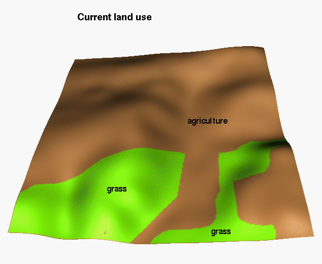


B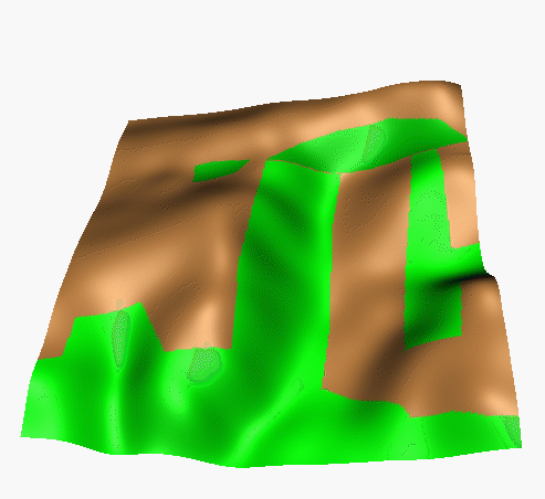


C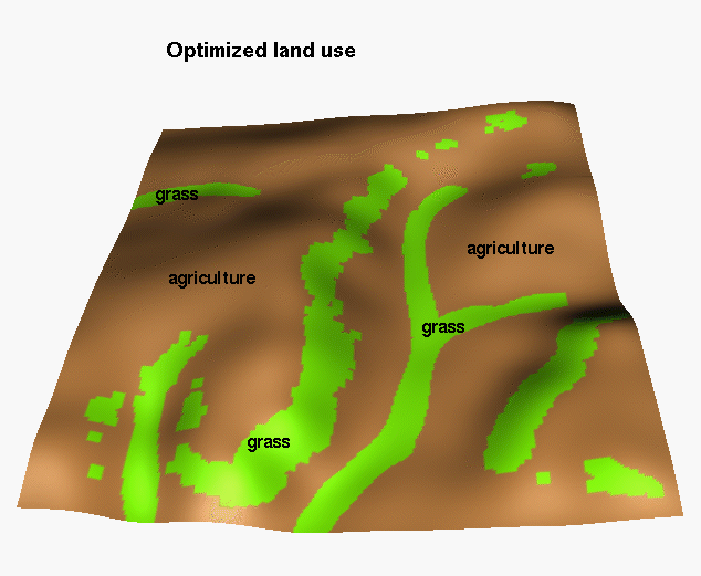
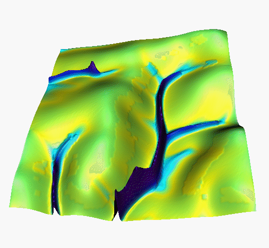


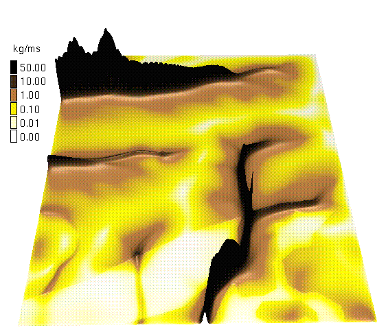
Figure 8. Evaluation of 3 different land use alternatives : Simulated water depth, sediment flow rate and net erosion/deposition for the original (A 21% grass), new sustainable (B: 40% grass) and computer designed (C:19% grass) land use, for the time of the year when the agricultural land (brown) is bare and grass cover(green) is well developed .
The vegetation growth during the year changes the properties of soil surface including its roughness with profound impact on water and sediment flow and pattern of erosion and deposition. The same land use can lead to different erosion/deposition patterns and sediment loads depending on the time of year when the storm event occurs. The following image shows that the difference between the roughness of two different covers (scenario B, Figure 8) has a significant impact on the erosion/deposition pattern and areas which experienced erosion can become depositional areas during a different time of year.
Figure 9. Impact of difference in roughness for spatially variable cover (scenario B) where Kt=Kd=0.03/0.0003 for both cases and surface roughness increases in the area of bare soil while it remains constant for grass a) n=0.01/0.1, b) n=0.05/0.1
This fact can be even better illustrated by the following example where we have simulated an impact of a) extremely large event (140mm/h) and bare soil in agricultural fields (n = 0.01, Kt = 0.03, Kd = 0.003, b) small event (18mm/h) with dense cover (n = 0.1, Kt = Kd = 0.0003). The simulation is in agreement with the hypothesis suggested by Auerswald (personal communication) that the material is deposited in the valley during repeated small events and then part of the accumulated material is eroded during extreme events with conditions leading to prevailing detachment limited case of erosion when large transport capacity of flow is present.
 a
a 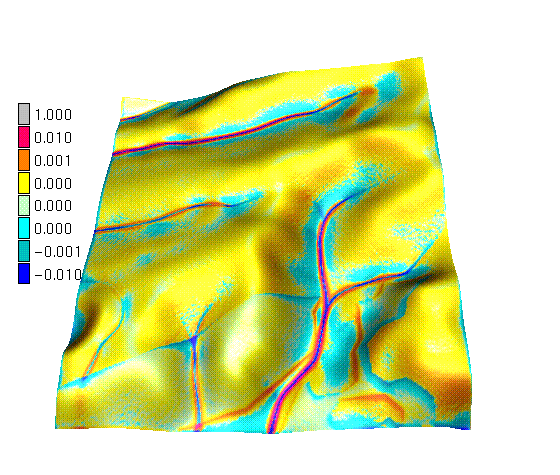 b
b
 c
d
c
d
Figure 10. Sediment flow a), c) and net erosion/deposition b), d) for a large a),b), and a small c), d) event for scenario A
We have tested the capabilities of the SIMWE model to simulate water flow and erosion processes for terrain with structures such as terraces and ponds, when terrain is not smooth and significant discontinuities and depressions are present. We have modified the terrain surface using standard GIS tools (r.digit, r.mapcalc, see the following chapter for more details) resulting in a surface with a simplified pond (depression) and a terrace (discontinuity-fault and a small flat area with zero gradient). For the test runs we have used a hypothetical case of uniform soil and cover, even on structures. The SIMWE algorithm was robust enough to simulate the water and sediment flow even for this complex situation, as illustrated by Figure 11, which shows water and sediment accumulation within the pond and a terrace. If the terrace wall is not enforced, as in our example, it will be rapidly eroded away. The results are encouraging and allow us to target the simulation of more complex and realistic structures in future (see also the simulation of a road impact in the previous report by Mitasova et al. 1996c).
Figure 11 Impact of terrain structures on water flow and net erosion/deposition under uniform conditions
Simulation of landscape processes is more sensitive to noise and artifacts in landscape characterization data than the more traditional uses of GIS such as automatic map production or spatial analysis. Efficiency of simulations depends on digital data representation where the traditional representation by polygons, commonly used for mapping, is not always the best approach for simulations. Also, the models often include complex spatial and spatio-temporal relationships and their understanding requires more sophisticated graphical representations than the standard 2D maps. Therefore, there is a continuing effort to extend the GIS capabilities to support modeling and simulation of processes (both within commercial products and research tools) by implementing new, advanced methods and data structures. Our effort has focused on improving methods for multivariate spatial interpolation, topographic analysis and visualization and extending the data structures to support multivariate point and raster format. Some of these improved capabilities will be available within the new GRASS releases in cooperation with the Baylor University GRASS Research Group (http://www.baylor.edu/~grass/).
Interpolation based on regularized spline with tension which has been enhanced and used for this project is described by Mitasova and Mitas (1993), Mitasova et al. (1995a,b), Mitasova et al. (1996). To gradually fulfill the requirements of spatial interpolation for GIS applications and simulations we are periodically enhancing the implementation of the RST method with the most recent enhancements including the support for spatially variable smoothing, which allows users to set a different smoothing parameter for each given point, depending on the accuracy of the measurement. This capability supports combination of data from various sources with different accuracies, with the resulting surfaces passing the closest to the most accurate data and allowing to deviate more from the data which are measured less accurately. We have also tested the interpolation tools in ArcView Spatial Analyst and found a serious flaw in the implementation and application of splines to a farm (crop yields, organic content, pH, etc.) used in the Spatial Analyst tutorial (ESRI 1997). We have provided the result of analysis to ESRI with suggestion to fix the flawed implementation of interpolation (Mitasova and Mitas 1997). The problem is being currently fixed.
Volume interpolation and visualization of soil data. To test the possibilities of creating 3D models of soil properties within a GIS we have computed a series of spatial models from comprehensive soil survey data for an experimental farm at Scheyern, Germany. Soil properties (data courtesy Dr. Auerswald), were measured in 3D space up to 1.2m depth and they included results of chemical analysis (pH, Nitrates, Phosphates, Potassium, Organic matter, etc.), soil texture analysis, and qualitative information for each sample. Using this data, it was possible to derive additional information and parameters such as the depth of colluvial deposits and hydraulic conductivity, needed for erosion simulations. From the point of view of spatial modeling a special challenge for representation and visualization of soil data poses the fact that the vertical spatial variability requires resolutions much higher than the resolutions used for the representation of phenomena in a horizontal plane. We have investigated various approaches to create a 3D model of the measured soil properties (Brown et al 1997), in particular by: a) sorting the data by horizons, interpolating a 2D raster map for each horizon at 2m resolution and creating a multiple surfaces model (Mitasova et al. 1996b); b) interpolating the 3D data to 3D raster map with 2m horizontal and 0.1m vertical resolution using the trivariate implementation of the RST method (Figure 12). To visualize vertical relationships with sufficient detail, we have used 100 times relative exaggeration of depths both for multiple surfaces representing the soil horizons (depths exaggerated relative to terrain surface) and for the series of volumetric data. The results are illustrated in this report by volume models of organic carbon, hydraulic conductivity and soil reaction (pH) combined with contours (Figure 12). We have found, that if the adequate tools are available, the full 3D model is more appropriate than the representation based on multiple surfaces as it incorporates the vertical relationships into interpolation and allows more efficient visual analysis. The 3D spatial model of organic carbon shows that its highest concentrations are in the area with long term grass cover. However, as expected, the amount of organic carbon rapidly decreases with depth (Figure 12a). The pH model shows greater spatial variability in vertical direction as the highest acidity on terrain surface, located in grass area, extends over larger area in deeper horizons (Figure 12c). The values of hydraulic conductivity were derived from information on particle size distribution for each sample. The interpolated 3D raster (Figure 12b) together with a DEM can be used as an input for 3D infiltration model, enhancing the realism of hydrologic simulations. Example of size fraction analysis visualization for points and a volume model of clay content is presented in Brown et al. (1997) including the results for nitrates, phosphates and other chemicals.
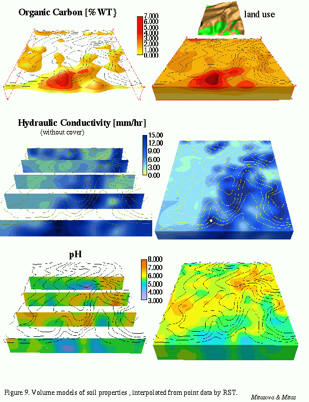
Figure 12. Soil chemical analysis and texture
Simplified structure design using standard GIS tools. Standard GIS tools, such as r.digit and r.mapcalc can be used to modify the terrain to include various man made structures, such as roads, ponds or terraces for the purpose of simulating impact of anthropogenic features on landscape scale erosion processes. The following procedure can be used to to add a simplified pond:
- display background info (terrain, water flow, rills,
etc),
- use r.digit to outline the structure (pond2.mask)
with depression as category 1, dam as category 2,
- use r.mapcalc to create depression and dam for
a simplified pond with horizontal bottom:
pond2.el = if(pond2.mask,pel.2m)
pond2.dig = 1.5+pond2.el-461.3 (pond with min.depth 1.5m)
- run r.support to change no-data to 0 (pond2.mask)
- use r.mapcalc to add the structure to terrain
surface
pel.pond2a = pel.2m-pond2.dig
Similar simple procedure can be used to create a terrace. Both
structures can be added to the terrain with the result illustrated in
Figure 13. More complex structures are possible by developing the
appropriate geometrical operations using r.mapcalc or by
designing interactive surface design tools operating on raster data.
Structures can be also imported from CAD tools or other software,
transformed to raster representation and used to modify the terrain,
however appropriate interface or import/export tools need to be
developed.
 a
a 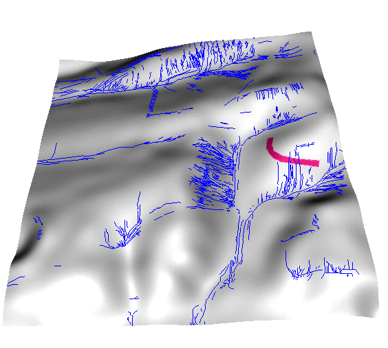 b
b  c
c
Figure 13. Original terrain, mask locating the terrace and resulting terrain surface
Besides increasing our knowledge about erosion processes in landscapes
the goal of this project is to develop methods and tools for erosion
risk assessment and erosion prevention support for military
installations. This task poses a special challenge, because military
installations occupy large areas with terrains much more complex than
typical agricultural regions for which most of the traditional erosion
modeling tools were developed. Also the landuse at installations often
combines relatively well preserved natural areas with landscape exposed
to high intensity disturbance, well beyond the impact of agriculture.
Therefore the principles of process based erosion modeling developed
for agriculture have to be significantly enhanced and new approaches
have to be designed to meet this challenge. We have already tested some
of our approaches for areas at military installations (Yakima, Camp
Shelby extension) as described by Mitasova et al. (1996bc, 1995b). In
this report, we further demonstrate the developed methodology for
military installations at Ft. Irwin and Ft. McCoy.
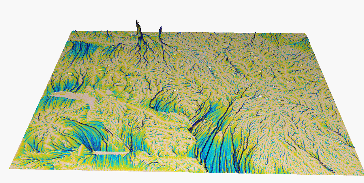
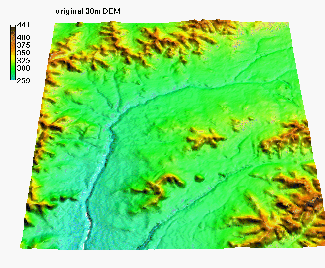
To illustrate the issues associated with simulations for large areas we use an example of a mountainous region in California. The standard 30m DEM available for the entire study area (3000 square km) represents 4 million grid cells, a challenging data set for the current process-based simulation tools and workstations, at the resolution hardly sufficient for rough identification of high erosion risk areas. The DEM at 5m resolution, needed e.g. for capturing at least approximately the effects of roads or grassways, would require to use data sets with 121 million grid cells and run simulations which would be prohibitively expensive, if not impossible with the current computational resources. It is clear, that for such a large area, modeling at different scales and resolutions is needed, depending on the importance and complexity of area's watersheds. It is important to note that our aim in this application is to illustrate the possibilities to use standard elevation data for erosion simulations in a large area. We are not taking into account the climate, soil and cover properties which certainly have a profound impact on water flow in this area. In spite of the fact that this is only a hypothetical example, this test allows us to assess the capabilities of our tools and prepare the environment for more realistic applications (e.g. Hohenfels installation).
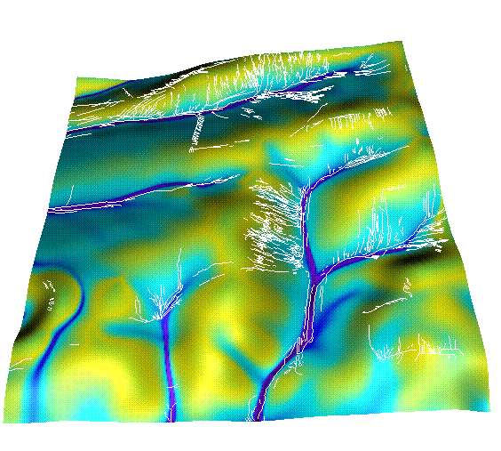
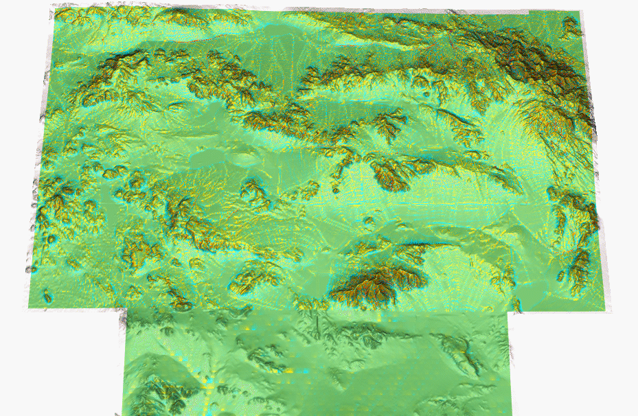
Digital elevation model and topographic analysis. To illustrate the issues of resolution, noise and systematic errors in standard elevation data we analyzed the 30m DEM available for Ft. Irwin (Figure 14) with more detailed analysis performed for the subareas A, B, C, D (Figure 15).
Figure 14. Fly-by over a DEM at Ft. Irwin

Figure 15. Topographic potential for soil detachment by water flow for entire Ft. Irwin with highlighted subares used for further analysis.
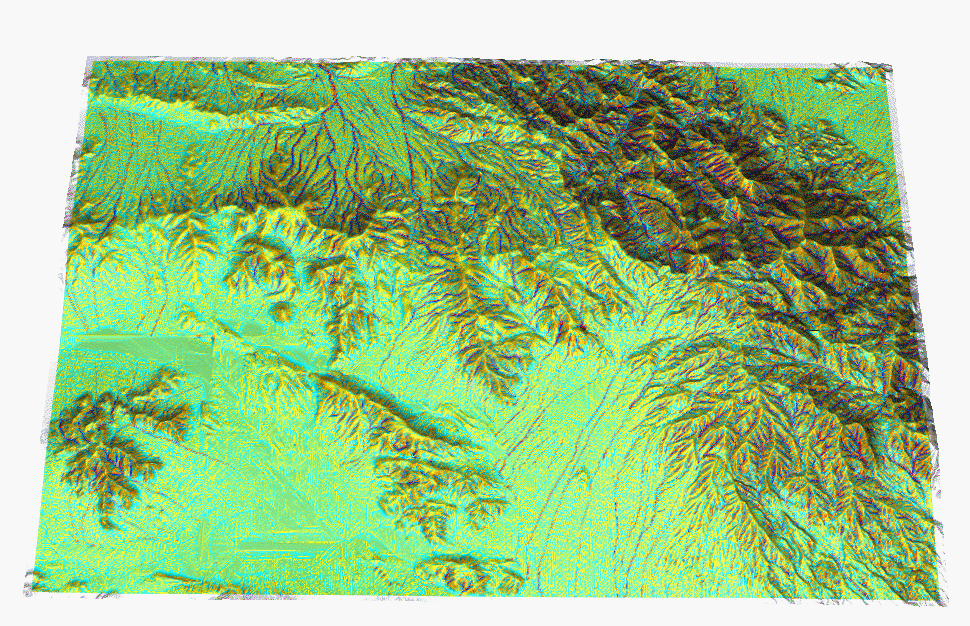
GRASS GIS allows us to compute several important topographic parameters describing various geometrical properties of terrain, as illustrated for an area C for the original 30m DEM:
Figure 16. Topographic parameters
Topographic parameters serve as inputs for erosion models but they are also useful for evaluating the quality of a DEM and identifying possible noise and systematic errors as illustrated by the following example of terrain with draped tangential curvature. Tangential curvature for 30m DEM shows acceptable structure in mountainous area while significant noise and systematic errors (stripes) are present in lowland (Figure 17a). After smoothing and resampling to 10m resolution using the RST interpolation method the noise is reduced and the major topographic features become more visible (Figure 17b):
 a
a  b
b
Figure 17. Terrain with
draped tangential curvature a) original 30m DEM and K_t , b) 10m DEM
and K_t with smoothing 1.0, ten=60
These images clearly demonstrate that the need for precision and accuracy is spatially variable, with flatter areas much more sensitive than mountains. Note how the artificial structure in flat areas continuously transforms into the real terrain structure in mountains. This is especially "dangerous" phenomenon if a DEM is going to be used for simulations, as the artificial structure can be mistaken for the real topographic feature.
Flow tracing is an important part of hydrologic and erosion modeling. The results are significantly influenced by flow tracing algorithm and resolution as well as quality of the DEM as illustrated by the following example, which compares the steady state water flow maps based on the original 30m DEM and the smoothed and resampled DEMs (Figure 18).
 a
a  b
b
Figure 18. Upslope
contributing area computed from a) original 30m DEM for area B, b) 10m
reinterpolated and smoothed DEM with smoothing 1., ten=60, area C.
Smoothing and resampling the original data with the RST reduced the artificial pits in the original DEM and allowed water flow to create continuous streams.
Topographic potential for erosion and deposition estimated by the USPED model. To illustrate the impact of smoothing and resampling on erosion modeling we have computed sediment transport capacity of water flow (Figure 19) and net erosion/deposition (Figure 20) at three resolutions: a) downscaled to 90m for the entire region, b) original 30m for a 500 square km subregion, c) smoothed and resampled to 10m for a 150 square km subregion. To demonstrate the differences in detail which can be achieved at various resolutions we have visualized the results as color maps draped over the 10m resolution DEM for a small subregion (36 square km). While the 10m resolution does not improve the accuracy of the original elevation model, the smoothing reduces the noise and high resolution allows better description of terrain geometry leading eventually to more realistic results of erosion model. The impact of noise and resolution is even more striking for modeling of net erosion/deposition (Figure 20) which is very sensitive to artifacts in a DEM as it is a function of second order derivatives (curvatures) of the elevation surface (Mitas and Mitasova 1997).
Figure 19. Topographic potential for soil detachment computed at different resolutions a) 90m, area A, b) 90m zoomed into area D, c) original 30m DEM, area B, d) 30m area D, e) reinterpolated and smoothed at 10m, area C, f) 10m area D.
 a
a b
b
 c
c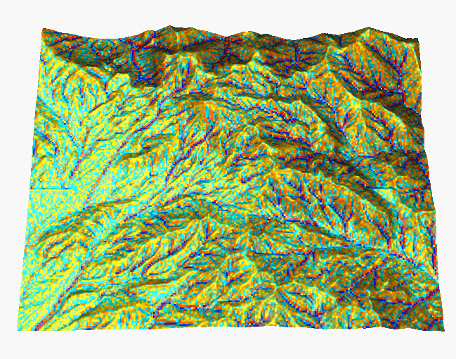 d
d
 d
d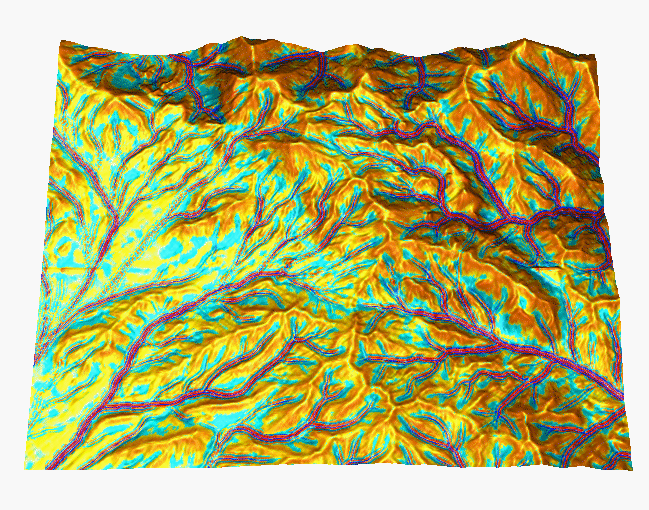 f
f
Figure 20. Topographic potential for net erosion and deposition computed at different resolutions a) 90m, area A, b) 90m zoomed into area D, c) original 30m DEM, area B, d) 30m area D, e) reinterpolated and smoothed at 10m, area C, f) 10m area D.
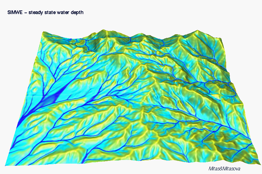
Water and sediment flow simulation by SIMWE. To test the applicability of SIMWE to areas significantly larger than the test Germany data we have computed the spatial distribution of steady state water flow, sediment flow and net erosion/deposition for a 36 square km subregion D (Figures 21, 23). This application demonstrates that processing of original elevation data by adequate tools, such as in our case the RST method and application of a robust, process-based model can lead to a significant improvement in predicted erosion/deposition pattern.
It is also possible to simulate approximately the dynamics of water
flow during a storm - the animation shows the development of water
depth during and after an uniform stationary storm which lasted approx.
5hrs (Figure 22).
Figure 22. Dynamic model of water flow depth during and after a uniform stationary storm.
Sediment flow rates are estimated by solution of continuity of mass equation using SIMWE showing high sediment flow rates in centers of valleys with dispersal of sediment flow in some areas (Figure 23a). Net erosion/deposition rates are estimated for a case with prevailing transport capacity limiting regime (Figure 23b). Note the disappearing and/or split gullies as the terrain flattens and alluvial cones are formed.
Figure 23. Spatial distribution of a) sediment flow b)net erosion/deposition rates for uniform soil and cover
The resampled and smoothed DEM and the results of simulation by the SIMWE model were provided for a development and demonstration of virtual reality tools for hydrologic simulations for CAVE at NCSA (Johnston and Reez, 1997) as illustrated by Figure 24. http://www.gis.uiuc.edu/hpgis/visualization.htm.
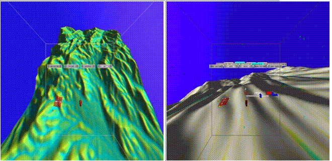
Figure 24. Virtual reality CAVE environment for exploration of hydrologic simulations.
We illustrate the estimation of topographic potential for erosion and deposition based on the USPED model using the elevation data provided at 30m horizontal resolution and 1m vertical resolution , for the following subarea of Ft. McCoy (Figure 25).
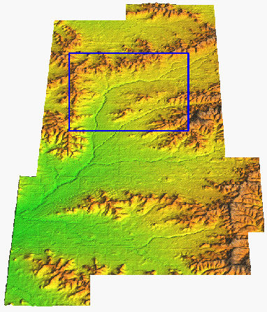
Figure 25. DEM for Ft.McCoy with highlighted test area.
Topographic potential for soil detachment and for net erosion and
deposition is estimated by the USPED model (Mitasova et al. 1996).
Even with rather crude elevation data, it is possible to identify the
areas with high topographic risk for soil detachment and
erosion/deposition, as illustrated by the following sequence of maps
showing the input 30m DEM (Figure 26a), intermediate steps (slope,
upslope contributing area, Figures 26b, 26c) and results of
computations (Figures 27a, 27b). Note the impact of plateaus in low
elevation areas on the slope pattern (artificial steeper slopes along
1m contours), highlighted by red arrows. These plateaus are due to the
insufficient vertical resolution of 1m. Upslope contributing area as a
measure of steady state water flow computed from the original 30m DEM
(Figure 26c) by r.flow is strongly underestimated. Pits
and plateaus in the DEM cause problems in flowtracing with almost no
flow generated in lower elevation areas and disrupted flow in valleys.
 a
a 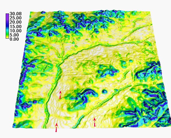 b
b  c
c
Figure 26. Inputs and intermediate results for
computation of erosion/deposition by USPED using original 30m DEM.
 a
a 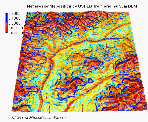 b
b
Figure 27. Topographic potential for soil detachment and net erosion/deposition computed by USPED using the original 30m DEM.
Modified LS factor predicts well some areas of high potential for soil detachment, especially in hilly parts of the region. However, it does not predict the location of areas with concentrated flow with high potential for rilling and gully formation . Also, in lower elevation areas the artificial pattern of increased erosion is predicted along 1m contours. The net erosion/deposition map computed by the USPED model predicts high net erosion in hilly regions and on slopes along the streams. It also shows that a significant portion of the material eroded from hillslopes is deposited before it could reach the main streams. However, this map lacks the prediction of high erosion due to concentrated flow in valleys and shows artificial waves of erosion and deposition along the 1m contours in flatter areas.
To reduce the negative impact of lower resolution of the available elevation data the given DEM was reinterpolated to 10m horizontal and 0.01m vertical resolution using the RST method. Simultaneously with interpolation, maps of slope, aspect, profile and tangential curvatures were generated (Figure 28).
 a
a  b
b  c
c
 d
d 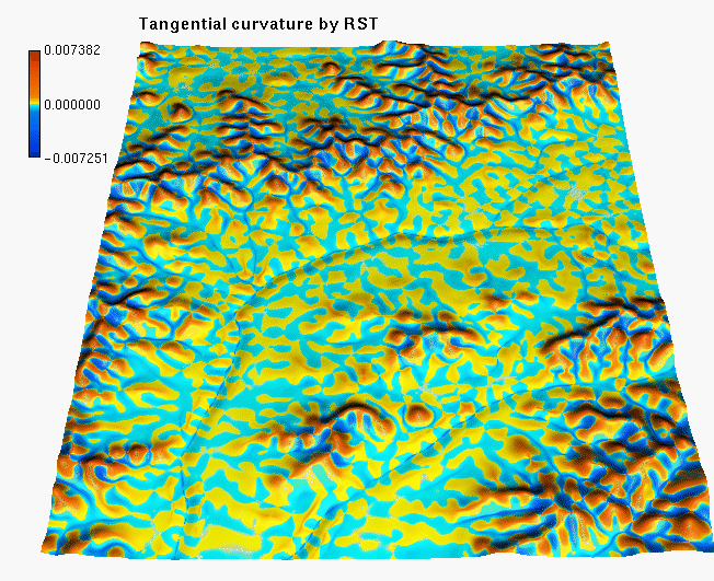 e
e
Figure 28. DEM reinterpolated to 10m resolution with simultaneous topographic analysis a) elevations, b) slope, c) aspect, d) profile curvature, e) tangential curvature.
Note, that in the slope map the artificial pattern of steeper slopes along 1m contours disappeared.

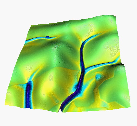
Figure 29. Steady state water flow.
Steady state water flow computed by r.flow from the smoothed 10m DEM shows potential for channel formation in valleys and predicts water flow also in low elevation region. Flow in the two main streams is not adequately described because of lack of data, but it can be incorporated if stream data are available.

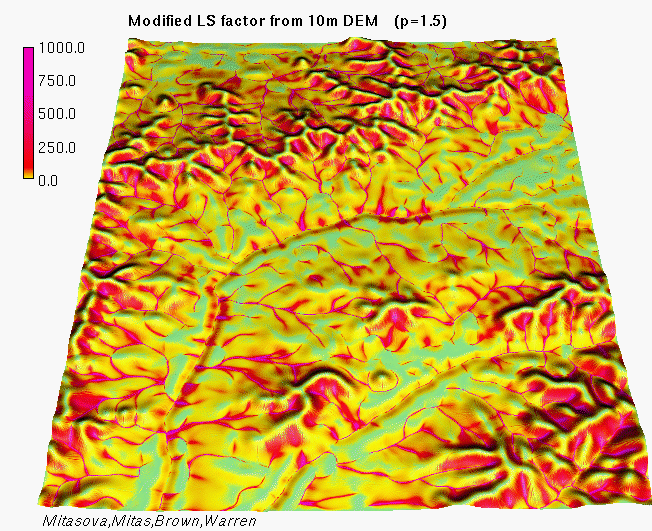
Figure 30. Modified LS factor or distribution of topographic potential for soil detachment by overland flow.
Modified LS factors were computed from the 10m DEM using different
exponents for the water flow term (p=0.6 and p=1.5).
Value of this exponent is still a subject of research and discussion in
erosion research community. The first result puts more weight on the
influence of slope while the second result puts more weight on the
influence of water flow. Because the exponent depends on the conditions
of water flow in a particular area it should be calibrated to reflect
the type of flow typical for the modeled area and time during the year.
. 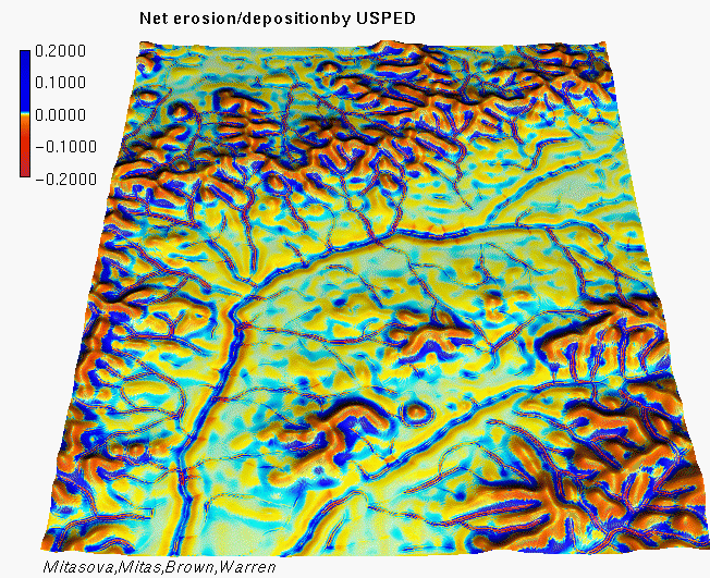
Figure 31. Topographic potential for net erosion/deposition computed by USPED
Topographic potential for net erosion/deposition was computed from the 10m DEM using the USPED model. Similarly as for the result of 30m DEM, the model shows high erosion in hilly area and along main streams and deposition in concave areas. It also indicates high erosion in areas with concentrated flow which could reach the main streams. The artificial pattern of erosion/deposition along contours is not present.
Impact of soil and cover will be incorporated when the land use/cover/soil categories or at least a rough estimate of C-factor are available. Also, estimation of sediment flow and net erosion/ deposition by process based distributed model SIMWE can be performed after we get data on land cover.
The presented approach and examples illustrate several aspects of advanced GIS application to landscape characterization and simulations of processes. We have demonstrated the importance of a proper choice of interpolation method when preparing the input data for simulations and the usefulness of smoothing and resampling of a standard 30m DEM to higher resolution for modeling of erosion and deposition. Replacing the geometry-based algorithms by physics-based models improves the flow related topographic analysis. Extension of GIS to 3D allows us to create spatial models which capture the distribution of phenomena in 3D space, however, anisotropic scaling and resolution is needed to create meaningful models. Implementation of concept of multivariate fields for landscape characterization data in GIS and development of appropriate supporting tools increases the efficiency of data preparation and of analysis and presentation of simulation results. This approach further supports the move from profile and/or polygon-based models, to full 3D dynamic simulations based on multivariate fields.
The stochastic method of solving the first principles equations using Green's function Monte Carlo technique provided us with a valuable research tool of a much needed robustness and flexibility. It enabled us to investigate several important issues such as erosion/deposition regimes, forms of sediment transport capacity and different landuse scenarios in a complex realistic landscape. Using the bivariate formulation, we have theoretically elucidated the observed relation between the pattern of erosion/deposition and the terrain shape in the transport capacity limited regime. In particular, we have shown the relation of terrain profile and tangential curvatures to the observed patterns and we have demonstrated that the impact of both curvatures is equally important for a proper description and understanding of erosion in 3D space.
A suggestion of Nearing at al (1997) that the sediment loads from rills may be more strongly influenced by a sediment transport limit rather than by the soil detachment, in general, agrees with our results. This seems to be true especially in complex terrain conditions where transport capacity changes significantly due to variations in terrain shape and cover affecting significantly the distribution and amplitudes of the water flow field. Our calculations and analysis also suggest that the sediment transport capacity plays a more important role than anticipated by the previous research which focused on erodibility as the key control quantity. Obviously, a subtle and spatially variable interplay between erodibility and transport capacity can influence the processes in a profound way. We believe that this complexity clearly points out towards the importance of the high accuracy-high resolution 2D simulations as one of the most promising research areas.
Arnold, J. G., P. M. Allen, and G. Bernhardt, 1993, A comprehensive surface-groundwater flow model. Journal of Hydrology, 142, 47-69.
Auerswald, K., A. Eicher, J. Filser, A. Kammerer, M. Kainz, R. Rackwitz,J. Schulein, H. Wommer, S. Weigland, and K. Weinfurtner, 1996, Development and implementation of soil conservation strategies for sustainable land use - the Scheyern project of the FAM, inDOPLN Land Use, edited by H. Stanjek,Int. Congress of ESSC, Tour Guide, II, pp. 25-68, Technische Universitat Munchen, Freising-Weihenstephan, Germany.
Bennet, J. P., 1974, Concepts of Mathematical Modeling of Sediment Yield, Water Resources Research, 10, 485-496.
Bjorneberg, D. L., Aase, J.K., Trout, T.J., 1997, WEPP model erosion evaluation under furrow irrigation. Paper no. 972115, 1997 ASAE Ann. Int. Meeting, Minneapolis, MI.
Brown, W. M., Mitasova, H., and Mitas, L., 1997, Design, development and enhancement of dynamic multidimensional tools in a fully integrated fashion with the GRASS GIS. Report for USA CERL. University of Illinois, Urbana-Champaign, IL. http://www2.gis.uiuc.edu/erosion/gsoils/vizrep2.html
Busacca, A. J., C. A. Cook, and D. J. Mulla, 1993, Comparing landscape scale estimation of soil erosion in the Palouse using Cs-137 and RUSLE, Journal of Soil and Water Conservation, 48, 361-67.
Desmet, P. J. J., and G. Govers, 1995, GIS-based simulation of erosion and deposition patterns in an agricultural landscape: a comparison of model results with soil map information, Catena, 25, 389-401.
Engel, B., Hydrology Models in GRASS, 1995, http://soils.ecn.purdue.edu:80/~aggrass/models/hydrology.html
ESRI, 1997, ArcView Spatial Analyst p 22-24, 59-60, 52-55
Flacke, W., K. Auerswald, and L. Neufang, 1990, Combining a modified USLE with a digital terrain model for computing high resolution maps of soil loss resulting from rain wash, Catena, 17, 383-397.
Flanagan, D. C., and M. A. Nearing (eds.), 1995, USDA-Water Erosion Prediction Project, NSERL, report no. 10, pp. 1.1- A.1, National Soil Erosion Lab., USDA ARS, Laffayette, IN.
Foster, G. R., and L. D. Meyer, 1972, A closed-form erosion equation for upland areas, in Sedimentation: Symposium to Honor Prof. H.A. Einstein, edited by H. W. Shen, pp. 12.1-12.19, Colorado State University, Ft. Collins, CO.
Foster, G. R., 1990, Process-based modelling of soil erosion by water on agricultural land, in Soil Erosion on Agricultural Land}, edited by J. Boardman, I. D. L. Foster and J. A. Dearing, John Wiley & Sons Ltd, pp. 429-445.
Foster, G. R., D. C. Flanagan, M. A. Nearing, L. J. Lane, L. M. Risse, and S. C. Finkner, 1995, Hillslope erosion component, WEPP: USDA-Water Erosion Prediction Project, edited by D. C. Flanagan and M. A. Nearing, NSERL report No. 10,pp. 11.1-11.12, National Soil Erosion Lab., USDA ARS, Laffayette, IN.
Garrote, L., and R. L. Bras, 1993, Real-time modeling of river basin response using radar-generated rainfall maps and a distributed hydrologic database, Report No. 337, pp. 15-180, MIT, Cambridge,.
Govers, G., 1991, Rill erosion on arable land in central Belgium: rates, controls and predictability, Catena, 18, 133-155.
Guy, B. T., Rudra, R. P. Rudra, and W. T. Dickinson, 1991, Process-oriented research on soil erosion and overland flow, Overland Flow Hydraulics and Mechanics, edited by A. J. Parsons, and A. D. Abrahams, Chapman and Hall, New York, pp. 225-242.
Haan, C. T., B. J. Barfield, and J. C. Hayes, 1994, Design Hydrology and Sedimentology for Small Catchments, pp. 242-243, Academic Press.
Hong, S., and S. Mostaghimi, 1995, Evaluation of selected management practices for nonpoint source pollution control using a two-dimensional simulation model, ASAE, paper no. 952700. Summer meeting of the ASAE, Chicago, IL.
Howard, A. D., 1994, A detachment-limited model of drainage basin evolution, Water Resources Research, 30(7), 2261-2285.
Johnston D., and Reez, W., 1997, 3D Visualization of Geographic Data using the CAVE. http://www.gis.uiuc.edu/hpgis/visualization.htm.
Julien, P. Y., and D. B. Simons, 1985, Sediment transport capacity of overland flow, Transactions of the ASAE}, 28, 755-762.
Julien, P. Y., B. Saghafian, and F. L. Ogden, 1995, Raster-based hydrologic modeling of spatially varied surface runoff, Water Resources Bulletin, 31(3), 523-536.
Kirkby, M. J., 1987, Modelling some influences of soil erosion, landslides and valley gradient on drainage density and hollow development. Catena Supplement, 10, 1-14.
Kramer, S., and M. Marder, 1992, Evolution of River Networks, Physical Review Letters, 68, 205-208.
Krcho, J., 1991, Georelief as a subsystem of landscape and the influence of morphometric parameters of georelief on spatial differentiation of landscape-ecological processes, Ecology(CSFR), 10, 115-57.
Maidment, D. R., 1996, Environmental modeling within GIS, in GIS and Environmental Modeling: Progress and Research Issues, edited by M. F Goodchild, L. T. Steyaert, and B. O. Parks, GIS World, Inc., pp. 315-324.
Martz, L. W., and E. de Jong, 1987, Using Cesium-137 to assess the variability of net soil erosion and its association with topography in a Canadian prairie landscape, Catena, 14, 439-451.
Martz, L.W., and E. de Jong, 1991, Using Cesium-137 and landform classification to develop a net soil erosion budget for a small Canadian prairie watershed, Catena, 18, 289-308.
Meyer, L.D., and Wischmeier, W.H., 1969, Mathematical simulation of the process of soil erosion by water. Transactions of the ASAE, 12, 754-758.
Mitas, L., and Mitasova, H., 1998, Distributed soil erosion simulation for effective erosion prevention. Water Resources Research, in press.
Mitas, L., Mitasova, H., 1997, Spatial Interpolation.In: P.Longley, M.F. Goodchild, D.J. Maguire, D.W.Rhind (Eds.),Geographical Information Systems: Principles, Techniques, Management and Applications (in press).
Mitas, L., Mitasova, H., 1997, Green's function Monte Carlo approach to erosion modeling in complex terrain. Paper No. 973066,1997 ASAE Annual International Meeting,Minneapolis, Minnesota.
Mitas L., Brown W. M., Mitasova H., 1997, Role of dynamic cartography in simulations of landscape processes based on multi-variate fields. Computers and Geosciences, Vol.23, No. 4, pp. 437-446 (includes CDROM and WWW: www.elsevier.nl/locate/cgvis).
Mitasova, H., Mitas, L., Brown, W.M. and Warren, S. 1997, Multi-dimensional GIS environment for simulation and analysis of landscape processes, Paper No. 973034, 1997 ASAE Annual International Meeting,Minneapolis, Minnesota.
Mitasova, H., Mitas, L., 1997, ArcView Spatial Analyst Spline Interpolation. http:http://www2.gis.uiuc.edu/erosion/esri/splinearc.html
Mitasova, H., Mitas, L., Brown, W. M., Johnston, D., 1996c, Multidimensional Soil Erosion/deposition Modeling. PART III: Process based erosion simulation. Report for USA CERL. University of Illinois, Urbana-Champaign, IL,pp. 28.
Mitasova, H., W.M. Brown, D. Johnston, L. Mitas, 1996b, GIS tools for erosion/deposition modeling and multidimensional visualization. PART II: Unit Stream Power-Based Erosion/Deposition Modeling and Enhanced Dynamic Visualization. Report for USA CERL.University of Illinois, Urbana-Champaign, IL, pp. 38.
Mitasova, H., J. Hofierka, M. Zlocha, and R. L. Iverson, 1996a,
Modeling topographic potential for erosion and deposition using
GIS,Int. Journal of Geographical Information Science, 10(5), 629-641.
(reply to a comment to this paper appears in 1997 in Int. Journal of
Geographical Information Science, Vol. 11, No. 6)
Mitasova, H., Mitas, L., Brown, W.M., Gerdes, D.P., Kosinovsky, I., 1995, Modeling spatially and temporally distributed phenomena: New methods and tools for GRASS GIS. International Journal of GIS, 9 (4),special issue on integration of Environmental modeling and GIS, p. 443-446.
Mitasova, W.M. Brown, D. Johnston, B. Saghafian, L. Mitas, M. Astley, 1995, GIS tools for erosion/deposition modeling and multidimensional visualization.Part I: Interpolation, rainfall-runoff, Visualization. Report for USA CERL. University of Illinois, Urbana-Champaign, IL, pp. 45.
Mitasova, H., and L. Mitas, 1993, Interpolation by Regularized Spline with Tension: I. Theory and implementation, Mathematical Geology, 25, 641-55.
Mitasova, H., J. Hofierka, 1993, Interpolation by regularized spline with tension : II. Application to terrain modeling and surface geometry analysis. Mathematical Geology 25, p. 657-669.
Moore, I. D., and J. P. Wilson, 1992, Length-slope factors for the Revised Universal Soil Loss Equation: Simplified method of estimation, Journal of Soil and Water Conservation, 47, 423-428.
Moore, I. D., A. K. Turner, J. P. Wilson, S. K. Jensen, and L. E. Band, 1993, GIS and land surface-subsurface process modeling, in Geographic Information Systems and Environmental Modeling}, edited by M. F Goodchild, L. T. Steyaert, and B. O. Parks, pp.196-230, Oxford University Press, New York.
Nearing M.A., Norton L.D., Bulgakov D.A., Larionov G.A., West L.T., Dontsova K.M., 1997, Hydraulics and Erosion in eroding rills. Water Resources Research, 33, 865-876.
Quine, T. A., P. J. J. Desmet, G. Govers, K. Vandaele, and D. E. Walling, 1994, A comparison of the roles of tillage and water erosion in landform development and sediment export on agricultural land near Leuven, Belgium, in Variability in stream erosion and sediment transport, edited by L. J. Olive, R. J. Loughran, and J. A. Kesby, IAHS Publication, no. 224, Proc. of an Int. Symposium Canberra, Australia, pp. 77-86.
Rewerts, C. C. and B. A. Engel, 1991, ANSWERS on GRASS: Integrating a watershed simulation with a GIS. ASAE Paper No.91-2621. American Society of Agricultural Engineers, St.Joseph, Missouri, 1-8.
Saghafian, B., Implementation of a Distributed Hydrologic Model within GRASS, in {\sl GIS and Environmental Modeling: Progress and Research Issues}, edited by M. F Goodchild, L. T. Steyaert, and B. O. Parks, GIS World, Inc., pp. 205-208, 1996.
Srinivasan, R., and J. G. Arnold, 1994, Integration of a basin scale water quality model with GIS, Water Resources Bulletin, 30(3), 453-462.
Sutherland, R. A., 1991, Caesium-137 and sediment budgeting within a partially closed drainage basin, Zeitschrift Fur Geomorphologie N.F. Bd., 35, Heft 1, 47-63.
Vieux, B. E., N. S. Farajalla, and N. Gaur, Integrated GIS and distributed storm water runoff modeling, in {\sl GIS and Environmental Modeling: Progress and Research Issues}, edited by M. F. Goodchild, L. T. Steyaert, and B. O. Parks, GIS World, Inc., pp. 199-205, 1996.
Warren, S., K. Auerswald, L. Mitas, and H. Mitasova, 1996, Advanced tools for predicting soil erosion and deposition, paper presented at II. International Congress of European Society for Soil Conservation, Technische Universitaet Muenchen, Freisig-Weihenstephan, Germany, September.
Willgoose, G. R., R. L. Bras, and I. Rodriguez-Iturbe, A physically based coupled network growth and hillslope evolution model 1, Theory, {\sl Water Resour. Res.}, 27(7), 1671-1684, 1991.
Willgoose, G. R., R. L. Bras, and I. Rodriguez-Iturbe, A physically based channel network and catchment evolution model, technical report no. 322, Ralph Parsons Lab., MIT, Cambridge, Mass., USA, 1989.
All full size figures are available in electronic form as part of the electronic version of this report at: www2.gis.uiuc.edu/erosion/reports/cerl97/rep97.html
For illustration, we provide color hardcopies for the following selected figures:
Figure 1. Comparison of observed and predicted deposition pattern using 1D and 2D flow
Figure 2. Impact of increasing rainfall excess on erosion/deposition pattern
Figure 4. Impact of increasing critical shear stress on erosion/depostion pattern.
Figure 8. Simulation of water depth, sediment flow and net erosion/deposition for different land use alternatives.
Figure 12. Volume models of soil properties
 a
a b
b c
c a
a b
b a
a b
b c
c movie
movie movie
movie b
b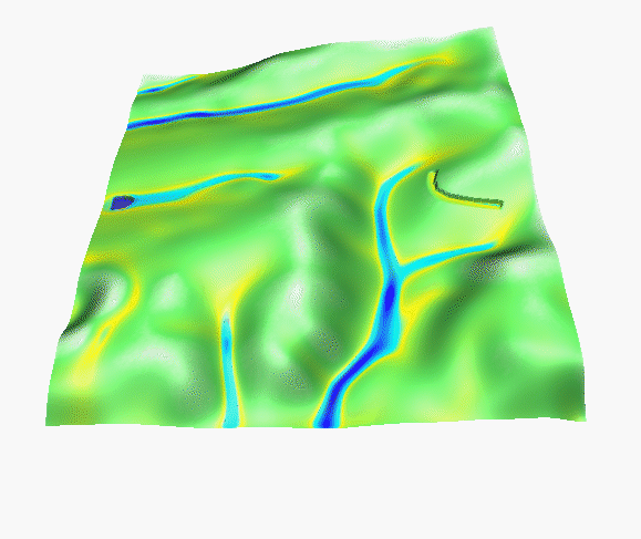 a
a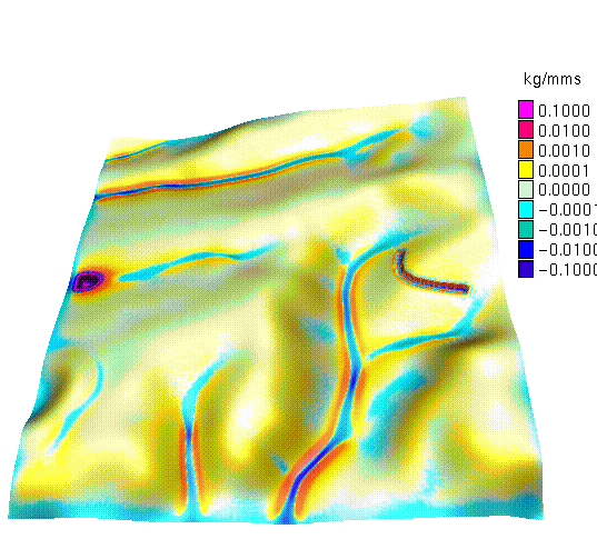 b
b a
a a
a 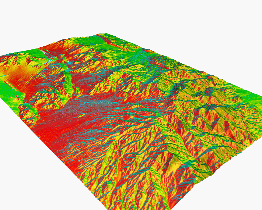 b
b  c
c  d
d a
a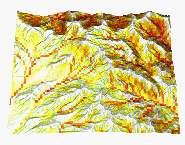 b
b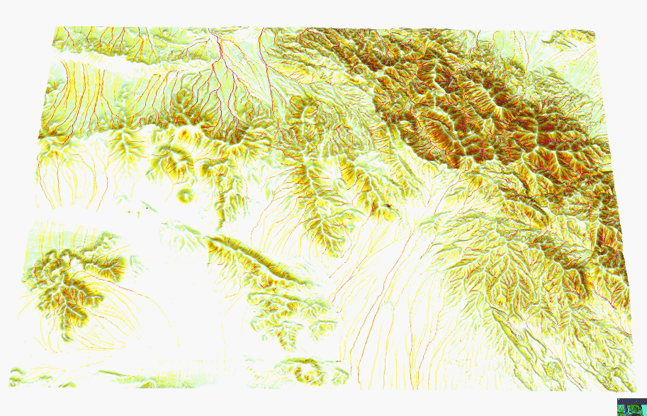 c
c  d
d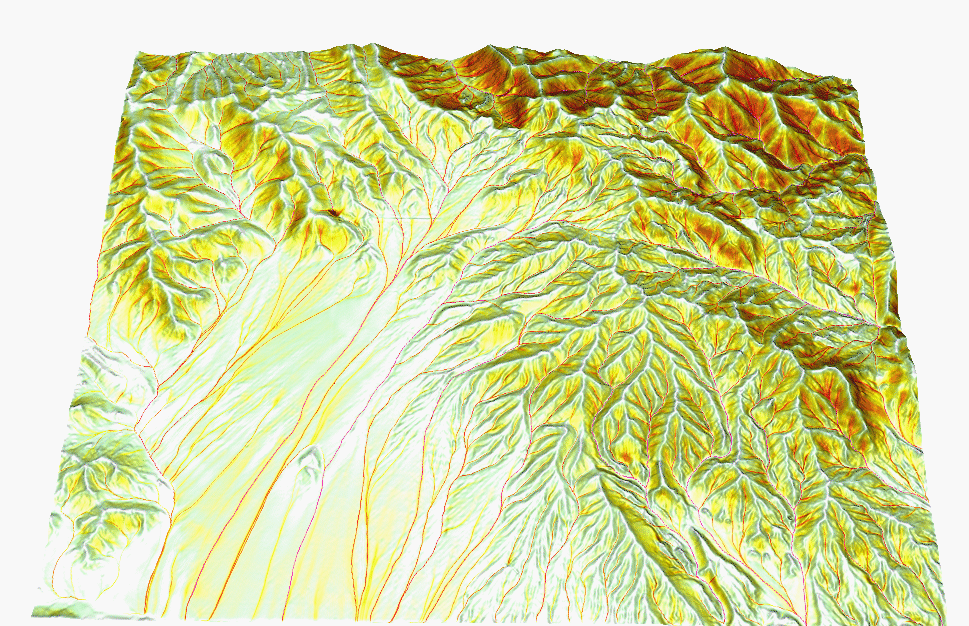 e
e  f
f movie
movie  a
a  b
b