Terrain modeling and Soil Erosion Simulation:
applications for evaluation and design of conservation strategies
Prepared by:
Geographic Modeling and Systems Laboratory, University of Illinois at Urbana-Champaign
Helena Mitasova, Lubos Mitas, William M. Brown, Douglas M. Johnston, GMSLaboratory
and Seuth Dabney, National Sedimentation Laboratory
for :
U.S. Army Construction Engineering Research Laboratories
Dr. Dick L. Gebhart
Matthew Hohmann
Annual Report
2000
1. Introduction........................................................3

2. Methods.............................................................4

2.1 New generation of geospatial data..................................5
2.2 Modeling of landscape processes at a hierarchy of scales...........9
2.3 Path sampling ....................................................10

3. GIS - based erosion modeling for conservation planning.............13

3.1 Landscape/watershed scale modeling................................13
3.2 Modeling high resolution effects of conservation measures.........14
3.3 GIS implementation and application issues.........................18

4. Applications.......................................................22

4.1 Fort Hood ........................................................23
4.2 Fort Polk ........................................................29

5. Conclusion and future directions...................................32

6. References.........................................................33

7. Appendix...........................................................34
1. Introduction
New mapping and environmental monitoring technologies generate large volumes of high resolution spatio-temporal data and offer unique opportunity to dramatically improve the land management, alleviate environmental pressures and preserve biodiversity. The major challenge for the rapidly evolving geographical information science is to provide methods and tools for effective use of these data for environmentally and economically sound land use management, with focus on proactive prevention rather than just remediation of environmental problems. Many areas face increased pressures from urban development and at the same time large resources are being invested in conservation efforts with significant uncertainties about their effectiveness. It is therefore crucial to speed-up the relevant landscape modeling and management research so that it can provide the tools to evaluate the impact of changes before they are implemented and to support design of new, effective conservation and pollution prevention strategies.
The landscape-scale land management strategies are extremely difficult to test experimentally because of the cost and time requirements of such experiments and because of limited possibilities to evaluate their functioning under extreme conditions. Laboratory experiments, while useful, often behave quite differently from large-scale real-world systems, thus limiting the applicability of their results. Field experiments can support the studies of certain properties of conservation measures, however, they are constrained both spatially and temporally and cannot capture the long-range interactions typical for fluxes in complex landscapes. One area of special promise to address these issues is simulation modeling which can give decision makers interactive tools for both understanding the system and judging how management actions might affect that system" (NRC, 1999)".
One of the key challenges in environmental modeling research is the description of interacting physical processes with sufficient accuracy and efficiency. It is clear, that a rapid development of computer technology offers new opportunities to tackle extremely complex environmental problems. In fact, computational simulation and modeling is becoming a third way of performing scientific research complementing the traditional experiments and analytical theories. Computational approaches belong to "young" methodologies which were developed only over the past few decades and their progress is closely tied to the advances in computer capabilities. As such, they have their own rules, challenges, successes and limitations. The role of algorithms, data structures, computationally efficient methods, advanced visualization and exploration of parallelism are crucial for new advances in environmental research and require close collaboration between traditional research disciplines and computational science.
Originally, GIS applications were focused on static spatial data processing, analysis and computer cartography. However, development of new geospatial data collection technologies and computer capabilities together with acute environmental problems have pushed the GIS applications into more sophisticated levels. Advanced geoscientific applications involve multidimensional phenomena (e.g., Mitasova et al 1995), dynamics (Burrough 1998, Mitas et al. 1997), supercomputing class simulations as well as real-time processing of huge amount of measured data (Catin and Fortin 2000). Nevertheless, the process-based modeling of the geospatial phenomena involves substantially more uncertainty than modeling in physics or chemistry. One of the key reasons is the above mentioned complexity of studied phenomena. The practical solutions then have to rely on the best possible combination of physical models, empirical evidence, intuition and available measured data. In physics, the accuracy is usually understood in a much stricter sense, because many fundamental laws are known over a broad range of scales in energy, distance or time. For example, Schrodinger equation describes the matter at the electronic level virtually exactly, that means, within spectroscopic accuracy of 6 to 12 digits. This is seldom the case in complex geoscientific applications where 50% differences between measurements and model predictions can be in many instances considered satisfactory.
In spite of significant progress in Geographical Information Systems (GIS) technology and environmental modeling (Goodchild et al. 1993, 1996, 1997, GIS/EM4 2000) there are persistent problems with accuracy and reliability of spatial simulations, preparation of data is often time consuming and running the models requires substantial expertise. Finally, the modeling efforts have focused on analysis of the current state and prediction, while their use for development of new land management and conservation strategies is largely unexplored.
In this report we address the issues of creating the digital representation of the landscape suitable for environmental modeling and simulations of processes, methodologies for robust multiscale modeling of landscape fluxes with focus on conservation planning and design, GIS implementation issues, and applications to military installations.
2. Methods
State of the art land use management is based on extensive use of GIS technology which provides tools for:
creating a digital model of the managed landscape with its features and properties
spatial analysis and identification of "hot spots"
spatial modeling and simulations
digital cartography and visualization
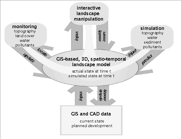
GIS supported model of the studied landscape provides the basis for landscape monitoring, analysis and simulation (Figure 1). To fully support land use management the landscape models should be created as a multi-resolution representation using the combination of a regional scale, low resolution model with embedded high resolution models for monitoring and simulation of "hot spots" (Mitas and Mitasova 1998b). Multiscale approach to land use management is supported by a new generation of high resolution geospatial data, robust and flexible simulation methods, such as path sampling, and process based models which adequatelly represent the phenomena important for conservation of natural resources.
Figure 1. GIS role in integration of landscape monitoring, analysis, planning and simulation.
2.1 New generation of geospatial data
New mapping and distribution technologies have dramatically increased access to geospatial data at unprecedented detail and coverage. However, the old problems with data consistency, reliability, seamless coverage have become a major obstacle for effective use of these data. In the following sections we describe some of the new GIS data that we had available, evaluate their suitability for modeling of landscape processes and identify the type of processing that may be needed to use these data effectively.
Digital elevation data While significant progress has been made in the development of digital elevation data, the DEMs remain the main source of problems when applying hydrologic and erosion models at landscape scale. Our experience as well as others (e.g., Heinzer et al., 2000) demonstrates that significant effort is needed for processing the DEMs before they can be used for modeling. We have evaluated the following elevation data:
a) USGS DEM at 10m resolution created by USGS from the same source as the 30m DEM, however more accurate interpolation was used and elevations are available with vertical precision of 0.1m rather than 1m, reducing the "step" effect. In spite of using the same data source the quality of this DEM is superior compared to the 30m DEM (see USGS documentation about the accuracy). Besides the increased precision, accuracy and resolution, the DEM provides much more detailed description of terrain features. Several new problems due to the TIN-based interpolation method were observed, such as waves along contours in steep areas (Fig. 2a,c), leading to artificial erosion/deposition pattern; noise, especially in flat areas, leading to noisy and inconsistent contours (Fig. 2b) and artificial dams in valleys due to triangulation. However the magnitude of these artifacts is much smaller than in previous models and it is within the DEMs accuracy. The negative impact on modeling results can be reduced by smoothing and/or reinterpolating the data.

a |

 b,c |
b) DEM from digital photogrammetry, at 5-10m resolution, usually derived from TIN, generated from aerial photography, by applying an appropriate interpolation method. The DEM that we obtained for Ft. Hood had vertical precision 1m, which is insufficient for correct estimation of slope pattern (and consequently also the erosion/deposition), especially in areas with relatively flat terrain. Moreover, the use of TINs in both cases creates artificial dams in valleys. This is a known problem of TINs and controlled triangulation should be used. The negative effect of insufficient vertical resolution can be partially reduced by reinterpolating the DEM. There is a dramatic difference between the distribution of slopes between the 1m integer DEM and floating point precision DEM derived from the same data (Figure 4.) The elevation data that we have obtained for Fort Polk were in the form of contours and TIN points so we have performed the interpolation using the RST method (see Mitasova et al. 1999). At 10m resolution the DEM usually includes natural depressions and flat areas and stream enforcement is not recommended, because it reduces the accuracy (USGS, personal communication) and removes an important terrain feature.
|
|
|
Figure 3. Histogram for a slope map a) original Ft. Hood 10m DEM has discrete distribution of slopes, with certain values of slope not represented at all, b) slopes from reinterpolated DEM have continuous distribution (see the consequences for erosion modeling in the application section).
c) IFSARE DEM was available for Ft.Hood. It was adequate for areas without vegetation, however it was unusable for vegetated landscapes (Mitasova et al 1999). A small sample of LIDAR data that we had available was insufficient for evaluation, however, based on literature (e.g. Heinzer et al. 2000) and personal communication with USGS, LIDAR provides the most accurate remotely obtained elevation data and should be evaluated for erosion modeling and conservation planning.
d) Rapid kinematic survey based on mobile GPS provides high resolution data with centimeters vertical accuracy. We obtained the sample data for a farm in Indiana (courtesy Kim Drackett) in the form of scattered data points, so interpolation was necessary to compute a DEM. This is a fast, efficient and accurate method for obtaining data with great detail for smaller areas - see example at (Mitasova et al. http://www2.gis.uiuc.edu:2280/modviz/pfar/farm1.html).
e) Direct field measurements by total station were by far the most accurate and detailed data that were available (see Mitasova et al. 1999) and for small areas where engineering structures for conservation need to be installed this type of measurements would be required.
It would be useful to test other types of DEM which land managers might have available to find out whether there is any type of DEM which would not require any preprocessing for erosion modeling from land managers.
Land cover The resolution and detail of new land cover data sets has greatly increased, compared to the widely available 30m land cover derived from Landsat imagery. For example, Fort Hood now has 1m resolution vegetation data, which represents a dramatic increase in spatial variability compared to traditional polygon based data (Figure 4a,b). It is therefore necessary to evaluate when such a detail is needed and when it can obscure large scale patterns and phenomena. Also the resolution does not always represent the spatial accuracy, for example - the classification procedure for the Fort Hood vegetation data used a 10m resolution DEM (so any spatial variability within the 10m which may be influenced by topography could be missed). Also, forests along streams were classified as alluvial forest based on a uniform distance from the stream, while in reality the width of the flood plain and its related vegetation greatly varies. We are currently comparing the high resolution vegetation data with the C-factor estimated for the soil erosion inventory performed by NRCS at Fort Hood and the first results indicate major differences, therefore further testing is needed to evaluate how these data need to be processed to provide reliable estimate of the C-factor.

a |
b |
Soils Comprehensive soil data in digital form are available from NRCS SSURGO database. The data are provided in polygon form, which means sharp boundaries between soil types. The database includes a large number of parameters and map layers representing the input parameters for erosion models, such as K-factor can be easily extracted (Figure 5).

Figure
5. K-factor draped over a DEM. It was derived from the polygon
soil map in ArcInfo and imported into GRASS as a 5m resolution
raster.
Rainfall We did not obtain any directly measured rainfall data therefore we used the R-factor from NRCS and data from literature (e.g., Haan et al. 1994). We have developed a methodology for interpolating rainfall data from meteorological stations with incorporation of topography and tested its accuracy for estimation of long term discharge averages in collaboration with researchers in Slovakia (Parajka et al., 2001). This method will be useful when the rainfall data from stations become available.
Erosion model parameters Some erosion model parameters are currently available on-line (see SedSpec, online RUSLE, etc.) and can be used if the installation does not have already such data available. However, these data usually have low resolution or are spatially averaged.
2.2 Modeling of landscape processes at a hierarchy of scales
Process-based modeling of geospatial phenomena is difficult and often involves a much higher level of uncertainty than, for example, simulations of microscopic systems in physics or chemistry which are based on virtually exact theories, such as quantum mechanics. Key reasons for these modeling difficulties are the complexity of landscape phenomena, the multitude of processes acting across a range of scales, non-equilibrium phenomena and/or lack of experimental data. The practical solutions rely on the best available combination of physical models, empirical evidence, experience from previous studies and available measurements. Landscape processes are therefore often described by a combination of physically-based and empirical models, and integration with field measurements using data adaptive simulation is especially important for increasing the reliability of predictions (e.g., Cantin and Fortin 2000). Typically, the physically-based models have the following components (Mitasova and Mitas, 2001):
Model constituents with corresponding physical quantities such as concentration, density, velocity, etc. In general, the physical quantities depend on position in space and on time and can be characterized either as fields, particles or ensembles of particles.
Configuration space and its range of validity for fields and/or particles. This includes specification of initial, external or boundary conditions, as well as physical conditions and parameters.
Interactions between the constituents such as impact of one field on another, interactions between particles and fields, etc.
Governing equations derived from natural laws which describe the behavior of the system in space and time. The typical examples are continuity, mass and momentum conservation, diffusion-advection, reaction kinetics and similar types of equations.
Many natural processes involve more than a single scale and exhibit multi-scale, multi-process phenomena (Steyaert 1993, Green et al. 2000). Many multi-scale problems can be partitioned into a hierarchy of effective models which are nested in the direction from fine to coarse scales. At a given scale the model incorporates simplified or "smoothed out" effects coming from finer, more accurate levels. In the direction from coarse to fine scales, one develops a set of effective embeddings which determine boundary and/or external conditions for the processes at finer scales. The fine scale processes are then modeled at high resolution only in "hot spots" of the studied system. Multiscale modeling in GIS can be performed using various approaches:
combination of a low resolution spatially averaged model (e.g. SWAT) applied at a regional scale with a high resolution distributed model (e.g. SIMWE) applied for selected hydrologic units - usually high risk subwatersheds or units with proposed use change,
nested grids - grids at a hierarchy of increasing resolutions,
irregular meshes with spatially variable density, such as TIN.
Nested grid approach is very well suited for implementation or link with GIS, because it relies on data structure which is standard and well supported within GIS. In our previous work we have proposed to use an alternative method to the traditionally used finite difference and finite element methods, called path sampling, which is well suited for nested grids implementation. Similar methods are known as path integrals in physics or random walks in stochastic processes (Gardiner 1985).
2.3 Path sampling
The path sampling is based on the fact that essentially any field can be represented by an ensemble of sampling points. For example, a scalar field can be determined by the distribution (spatial density) of sampling points in the corresponding region of space; conversely, ensembles of particles are often described by continuous fields. The duality of field <=> particle density is routinely employed in physics and helps to reformulate and solve complicated problems involving interacting systems with many degrees of freedom. The path sampling method has been successfully used in physics , chemistry, finance, etc., for linear or weakly nonlinear transport or time propagation problems which involve processes such as diffusion, advection, rate (proliferation/decay), reactions and others. It has several important advantages when compared with more traditional approaches. It is very robust, can be easily extended into arbitrary dimension, is mesh-free and is very efficient on parallel architectures including heterogeneous clusters of PCs and workstations. Path sampling is also rather straightforward to implement in a multi-scale framework with data adaptive capabilities. The method has been successfully used for distributed modeling of overland water and sediment flow and erosion/deposition studies (Mitas and Mitasova 1998), including multi-scale applications, and modeling of dissolved and suspended substances in lakes, estuaries and coastal areas (Dimou and Adams 1993).
Using the duality field <=> particle density, processes can be modeled as evolution of fields or evolution of spatially distributed particles (Fig. 7). We use the water and sediment flow simulation for a subwatershed at Hohenfels (Mitasova et al. 1999) to explain the basic principles of path sampling. First the source, in our case rainfall excess (rainfall - infiltration) is sampled with densities of particles representing the varying rate of rainfall excess (Fig. 6). Size of the path samples is selected based on the resolution / spatially variability of the source. Note higher density of particles in the disturbed areas with compacted soil and reduced infiltration.
|
|
|
Figure 6. Sampling of the rainfall excess source field by particles with density proportional to the rainfall excess rate.
These path samples are then propagated according to the function G( r,r',p) generating a number of sampling paths. Averaging of these path samples provides an estimation of the actual solution with statistical accuracy proportional to the number of walkers. The solution is not restricted to the steady state and the state of the modeled quantity at any given time can be obtained by averaging the path samples at that time.
|
|
b |
Figure 7. Path sampling solution of the continuity equation for water depth using duality between particle and field representation: a) water depth at 1 minute, b) water depth after 24 minutes. The grid is 416x430 cells at 10m resolution. Click on b) to see the animation.
Path sampling for sediment is more complex. When deposition occurs the size of the path sample (representing the mass associated with it) is reduced until the path sample diminishes. The rate of this process is controlled by the first order reaction coefficient. For sand (coefficient greater than 1), the particles move only for a short distance and deposit quickly, while for clay, (with the coefficient 0.001) the particles are transported over long distance (see Mitasova et al. 1998), (Figure 8). Path sampling was implemented in the SIMWE model which was recently was enhanced to output the temporal development of water and sediment flow in both its particle and continuous field representation, for the uniform and multiscale version. The spatio-temporal version was tested for Hohenfels and the results clearly demonstrate the negative impact of compacted soil by moving large amounts of water and sediment into the stream very quickly, compared to slow movement of water within the forested subwatersheds. While this is a known phenomenon, the animation (Fig. 7) from the model may serve as a powerful demonstration of the impact that the sediment transport of soils with fine particles can have on the streams.
 a |
 b b
|
Multiscale path sampling The multiscale approach is useful for high resolution modeling of "hot spots", such as locations undergoing substantial land use change or areas targeted for conservation measures. The implementation is based on a multipass simulation. First, the entire area is simulated at a lower resolution, and the walkers entering the high resolution area(s) are saved. The saved walkers are resampled by splitting each one walker into a number of "smaller" walkers which are randomly distributed in the neighborhood of the original walker. The model is then run at high resolution only for the given subarea, with the resampled walkers used as inputs (Fig.9). If several different land use alternatives are considered for the given subarea, this approach can be used to perform simulations for each alternative only within the high resolution subarea. The approach also provides useful spatial information about the locations where water flows into the given subarea and where it flows out (Fig. 9).
|
|
|
|
|
d |
Figure 9. Multiscale path sampling based on nested grids: a) samples at the start of the low resolution simulation, b) low resolution samples after 25 minutes, with samples which reach the high resolution area shown in darker blue color, c) initial state of high resolution simulation with larger number of smaller particles, d) high resolution samples after 15 minutes. (Click on the last image to run animation)
3. GIS-based erosion modeling for conservation planning and design
GIS plays a fundamental role in state-of-the art landscape-scale conservation planning. While design of individual conservation measures, such as ponds, dry dams, grassed waterways is well served by CAD software tools and a specialized engineering software, landscape-scale planning requires a broader view of the spatial relations which is better supported by a GIS. GIS allows to import, process and analyze geospatial data from a wide range of sources, such as remote sensing, digitized maps, field measurements and get a synergistic view of the studied landscape and its components.
3.1 Landscape/watershed scale modeling
While spatially averaged models are useful for identification of high risk hydrologic units they are not very well suited for conservation planning, and fully distributed models are needed to support this task. At the landscape scale the goal of modeling is to identify areas with high erosion risk due to the combination of insufficient land cover and terrain configuration (steep slope, convex terrain shape or convergent topography), and evaluate general conservation strategies such as implementation of stream buffers and selection of large conservation areas in high risk locations. Fast and efficient approach is to use the models which represent limiting case of erosion regimes and are simple to compute in GIS by combining the flow-tracing and topographic analysis functions with map algebra. They can be applied to a single storm, monthly and annual estimates of soil detachment and net erosion/deposition. Various versions of the RUSLE model modified for complex topography (RUSLE3d) can be used to estimate soil detachment pattern (Mitasova et al. 1999, Desmet and Govers 1996), while the USPED model identifies the potential of landscape for net erosion and deposition. Both models use readily available parameters and can provide valuable spatial information about: (i) the location of areas with high erosion risk from both shallow overland and concentrated flow, (ii) relative estimates of erosion and deposition rates for different land use alternatives and conservation strategies. Locations identified as high risk from both RUSLE3D and USPED should be primary targets for field erosion inventory (to validate the risk) and implementation of prevention/mitigation measures (if the high risk is confirmed in the field). Computation of net erosion and deposition is also useful for evaluation of the landscape's capacity to deposit the eroded material before it can reach the streams. Erosion from concentrated water flow is not very well integrated in the traditional models. RUSLE3d and USPED can identify the areas with this type of erosion, and we are using the data from erosion inventory at Fort Hood to develop suitable parameters which will provide adequate quantitative estimates of concentrated flow erosion from these models.
A practical example of distributed watershed scale evaluation of conservation strategies in a Illinois watershed (see Appendix or http://www2.gis.uiuc.edu:2280/modviz/courtcreek/lhu52/cctable.html) compares the erosion risk and net erosion/deposition pattern for :
uniform row crop agriculture of entire watershed,
stream buffers with uniform width,
combination of stream buffers and conservation areas on steep slopes and
model based design of critical conservation areas
current land use
The analysis shows that the watershed has very good, conservation-oriented land use and soil loss can be further reduced by focusing on headwater areas and concentrated flow erosion. The comparison has also demonstrated the problem of relying only on buffers in watershed management. The riparian buffers are often designed based only on the distance from the streams neglecting the impact of topography, especially the areas with convergent water flow. Results from models indicate that increased water and sediment flowing from intensively used uplands can get through the buffers because of unprotected headwater areas which allow the development of concentrated flow. While the benefit of riparian buffers for the stabilization of the riparian area and reduction of sediment and pollutant loads delivered to streams is well known, the modeling results show that the buffers are often too narrow and offer surprisingly small benefit for the stability of the entire watershed unless at least steep slopes and concentrated flow areas are well protected.
3.2 Modeling high resolution effects of conservation measures
Conservation measures reduce erosion, restrict sediment transport and prevent sediment pollution by reducing runoff, soil detachment and transport capacity of overland flow and by trapping the transported sediment. The long term effectiveness of conservation measures depends upon complex interactions and to capture these interactions at a sufficient detail, process-based distributed models are needed. We have evaluated the suitability of SIMWE for simulation of some well know effects of conservation measures so that the missing capabilities could be identified and developed and the benefit of simulations for effective design of conservation measures can be evaluated.
Based on the landscape-scale analysis of erosion risk, which identified the concentrated flow erosion as one which has insufficient modeling and conservation support, we have studied the conditions for the development of concentrated flow erosion and the effectiveness of grassed waterways for its prevention. Development of high erosion in areas of concentrated flow was studied by performing simulations of water flow and net erosion deposition for an experimental field with uniform land cover (350x270m, modeled at 2m resolution; Zhang, 1999, Mitasova et al. 1999). For a short rainfall event ending before the flow has reached steady state, the maximum erosion rate was on the upper convex part of the hillslope and there was only deposition in the center of the valley (Fig. 10a). As the duration of the rainfall increased, water depth in the center of the valley has grown rapidly until it reached a threshold when linear features with very high erosion rates developed within the depositional area, indicating potential for gully formation (Fig. 10b). This effect can be modeled by both USPED (Mitasova et al., 1996, 1999) and SIMWE (Mitas and Mitasova, 1998), however, a smooth, high resolution DEM without artifacts is needed to realistically capture this commonly observed phenomenon (see Fig. 2c in Mitas and Mitasova, 1999). Increase in the roughness in the field "delays" the onset of erosion in the center of the valley by making the water flow "ridge" wider and lower. Uniform increase in the density of vegetation can play an important role in reducing the risk of gullies and the simulations can help to find the surface roughness/vegetation density which has to be maintained to prevent gully formation for the given rainfall intensity and duration.
|
|
|
|
|
|
Figure 10. Water depth and net erosion/deposition pattern for 18mm/hr rainfall excess for a) short event, with only deposition in the valley center, b) long event leading to steady state flow, with both high erosion and deposition in the valley center, indicating a potential for gully formation c) long event (steady state) with bare soil, d) steady state with dense vegetative cover. The 350x270m field is modeled at 2m resolution.
Grassed waterways. The common practice for prevention of erosion by concentrated flow are grassed waterways. Their design is guided by the topographic conditions and roughness within the grassed area, represented by Mannings coefficient. To investigate the impact of a grassed waterway, the water and sediment flow as well as net erosion/deposition pattern were simulated for a field within the Scheyern experimental farm (Auerswald et al., 1996; Mitas and Mitasova, 1998) for the bare soil conditions and after the installation of grassed waterway with different values of roughness in the field. For the bare field, there is a potential for gully formation (Fig. 11a). After the installation of grassed waterway the center of the valley becomes a depositional area. However, if the roughness in the field is several times smaller than in the grassed area, high erosion develops around the waterway, potentially replacing one big gully with two smaller ones. This "double channeling" problem can substantially increase the cost of the waterway maintenance (Fig. 11b). Increasing the roughness in the field reduces the risk of double channeling and the transition from erosion in the field to deposition in the grassed area is relatively smooth (Fig. 11c). An alternative solution combines contour filter strip on the upper convex part of the hillslope with grassed waterway (Mitas and Mitasova, 1998).

Figure 11. Impact of grassed waterway and differences in roughness on sediment flow: a) bare field with gully potential in the center, b) grassed waterway (light grey, n=0.1) and the bare field ( dark grey, n=0.01) with sediment flow along the grassed waterway (double channeling), c) grassed waterway (n=0.1) and the field with increased roughness (n=0.05) without increase in sediment flow along the waterway and smooth transition from erosion to deposition.
Benching effect of hedges has gained an increased interest as a cost effective alternative to more complex terraces. Hedges are about 1-1.5m wide strips of dense vegetation installed along contour lines and the field data suggest that the combination of water erosion and tillage leads to natural creation of terraces along these hedges (Fig. 12, Dabney et al., 2000). Modeling the impact of hedges poses a special challenge - the deposition is observed within and above the hedges which means that backwater effect is present, erosion is observed below the hedges due to the cleaner water coming from hedges. Moreover, increased deposition above the hedges is observed in swales with convergent flow and increased erosion is observed on noses with dispersal flow. Interaction of these complex phenomena make it difficult to predict these effects using the traditional approaches based on 1D flow over predefined hillslope segments and a 2D continuous diffusive wave approximation which incorporates also the terrain change is needed.
|
|
|
Figure 12. Change in the topography measured 3 years after the hedges were installed at a National Sedimentation Laboratory's experimental field (Dabney et al, 2000).
|
|
|
|
|
|
Figure 13 Simulation of erosion/deposition patterns on a hillslope with hedges: a) with big difference in roughness erosion occurs above and bellow the hedge (this is used to divert runoff - see Dabney et al. 2000), b) with small difference in roughness deposition above and erosion bellow the hedge creates a terrace, c) without tillage rilling will develop between and through the hedge.
We have used a time series of SIMWE (Mitas and Mitasova 1998) simulations which included the change of terrain due to erosion and deposition, to evaluate the suitability of the model for predicting the functioning of hedges. Terrain and erosion/deposition pattern development after 7 steady state events with uniform rainfall excess 36mm/hr, and Mannings n=0.2 (hedge) and n=0.15 (field) results in deposition above and within the hedge and erosion below the hedge (Fig. 13b). The impact of swales and noses is also correctly simulated due to the use of 2D flow in simulation. These results are preliminary and are used to further develop the model so that the dynamics during the event as well as the temporal change in terrain can be properly simulated. The third example (Fig. 13c) shows the same simulation as in (Fig. 13b) with a reduced diffusion term and without smoothing of the new elevation surface between the events. After 7 events, rill-type features developed in the lower part of the hillslope in swales. This example confirms the importance of tillage and other smoothing processes between the events for the successful development of benches.
3.3 GIS implementation and application issues
There have been substantial changes in both ESRI products, which are used at DoD, and GRASS GIS over the past year. We briefly describe some of the changes and their impact on erosion modeling and conservation planning.
Erosion modeling using a new generation ArcGIS software tools. The GMS laboratory was approved as a beta testing site for a new generation of ESRI products ArcGIS giving us the opportunity to evaluate the best strategy for implementing the erosion models within the changing structure of the ESRI software.
The ArcGIS 8.1 software contains new versions of ArcView, ArcEditor, ArcInfo, and ArcGIS Extensions, all of which are licensed separately. Various ArcGIS applications (such as the three core applications; ArcMap, ArcCatalog, and ArcToolbox) run on top of the base ArcGIS software (ArcView, ArcEditor, or ArcInfo).
ArcGIS is scalable in that ArcView contains minimum data development or built-in analysis tools, ArcEditor adds additional data format handling and multiuser support, and ArcInfo adds the complete set of ESRI analysis tools. The extensions operate with the entire line of ArcGIS - e.g., Spatial Analyst may be used whether you are running ArcView or ArcInfo - there is no longer a need to license ARC GRID for ArcInfo, as the functionality is built into Spatial Analyst. The minimum configuration to run the developed GIS-based erosion models is ArcView with the Spatial Analyst extension. The application used is ArcMap, which has similar appearance and functionality of ArcView 3.2.
Although ArcView 3.2 contained a rudimentary graphical interface for building model networks, called ModelBuilder, the prerelease version of ArcGIS does not contain any such tool. The ModelBuilder interface in ArcView 3.2 was not sufficient to implement an erosion model however. If an improved version of this tool is planned for inclusion in future releases of ArcGIS, it may be capable of providing an easier way to run the model, by simply calling up a saved model network and changing the data and parameters.
In absence of such a modeling tool, ArcGIS provides built-in Visual Basic for Applications, which could be used with ArcObjects to build a complete interface for the models, based on the standards defined by LMS or other relevant DoD program.
For comparison, we provide the RUSLE3D calculation using ArcGIS 8.1, ArcMap
Given data

grid: elevation, K, C, (P)

constant: R=120, resolution=10

Computation

1. Enable Spatial Analyst

   under View... Toolbars  select Spatial Analyst

2. Calculate Slope

   from the Spatial Analyst toolbar, select Surface Analysis... Slope

   give the new theme name slope

3. Raster Calculator

   from the Spatial Analyst toolbar, select Raster Calculator

   build an expression:

   FlowAccumulation(FlowDirection([elevation]))

   Evaluate

   make the new theme permanent and change the name to flowacc

   build an expression in the Raster Calculator:

   Pow([flowacc] * resolution / 22.1, 0.6) * Pow(Sin([slope] * 0.01745) / 0.09, 1.3))

   Evaluate

   make the new theme permanent and change the name to lsfac

   build an expression in the Raster Calculator:

   R*[K]*[C]*[P]*[lsfac]

   Evaluate

   make the new theme permanent and change the name to soilloss
Compared to older versions of ArcView with Spatial Analyst, the new release has more intuitive map algebra and the computation is simpler and in fact closer to the GRASS implementation. The implementation of USPED still needs to be tested especially for the problem with floating point data being lost during the computation. We have compared the implementation of RUSLE3d in ArcView (Mitasova et al. 1999) with the methodology used at the Purdue University (Engels 2000). The implementations are similar and both had the same problems with the lack of full support for floating point data in older versions of ArcView. The development of Interface should be coordinated with other projects to minimize the need for land use managers to learn new environment for every application they need.
Open source GIS implementation with the new GRASS5. There has been a fundamental change in the development, maintenance and support of GRASS GIS after it was given the General Public License (GPL) and become the part of the Open source software infrastructure. Significant new tools and enhancements developed all over the world were added and GRASS GIS capabilities were substantially enhanced by links to additional Open source tools, such as R statistical language and PostgreSQL database system (Bivand and Neteler, 2000). As a research and development tool for new geospatial technologies GRASS is becoming an important addition to the existing commercial systems. It contributes to the rapidly growing open source geospatial computing infrastructure and benefits from modifications and enhancements by international team of GIS developers. As opposed to the ArcGIS, which is restricted to Windows, GRASS is available for UNIX, LINUX, MacOS X, and Windows making it a suitable option for a multiplatform environment. We continue to use GRASS as our main research tool. Implementation of the approaches that are tested and ready for routine use within the commercial software used in DoD is becoming easier with the capabilities of commercial software to better link with external tools. The core implementation of RUSLE3d and USPED in GRASS GIS has been outlined by Mitasova et al. 1999. While this implementation remains in principle the same for the new release, the preparation of data, analysis of results and communication of outputs is greatly enhanced by a new interface, viewing and analysis tools.
Resampling of a DEM. In spite of a significant progress in topographic mapping the DEMs which are available from the government agencies or contractors often require further processing to make them suitable for modeling (see section 2.1). One of the common tasks is the resampling and smoothing of a DEM to reduce noise and artifacts from the measurements and inadequate processing. The following procedure can be implemented in any GIS which has tools for random point sampling and a suitable spatial interpolation with smoothing capabilities. In GRASS GIS the DEM is first transformed to randomly distributed points using the command r.random, with the number of points depending on the resolution and complexity of the terrain surface (usually 1 sampling point per 2-4 pixels). Then, the DEM is reinterpolated from these point data using the command s.surf.rst with carefully selected tension and smoothing. The number of representative samples can be optimized by interpolating the DEM with increasing number of samples until any increase of samples does not bring any difference in the resulting surface. Additional point data can be added to improve the resulting DEM such as points along the streams, and different densities can be used for different subareas by applying the r.random for different g.region settings. The proper selection of tension and smoothing parameters is crucial, unfortunately the crossvalidation version of s.surf.tps has not been yet ported to GRASS5, so the parameters have to be estimated empirically. In case that the impact of integers in the original DEM needs to be minimized it is useful to generate contours at 1m interval, transform them to sites by v.to.sites and interpolate, rather than use r.random which will preserve the flat areas that we are trying to reduce. The impact of resampling on slope computation and erosion estimates is illustrated by Figure 3. and Figure 18. The resulting smoothed DEM can then be used with the erosion models described in Mitasova et al. 1999 or other models outside the GIS.
Post-processing, visualization and design To make the results of models useful for land use management and decision making, it is important to provide tools which will allow the user to create meaningful maps and numerical reports in terms relevant to the planning task. Visualization plays an important role for evaluation of the input data and results of simulations as described e.g., by Mitas et al. 1997, or in our previous reports Mitasova et al. 1998,99. Creating detachment and erosion/deposition maps is often difficult because the values are highly non-linear, change over several magnitudes and the results of models may be noisy. We have therefore developed color schemes which allow us to create consistent maps of the results from the models, in particular, maps of upslope area/water depth, detachment rate (RUSLE3d), net erosion deposition (USPED, SIMWE) and sediment flow rate. The color schemes are in the Appendix.
Because of the non-linearity it is useful to create categories for the resulting maps so that the histograms and reports can be generated e.g., by using r.report command in GRASS. As described in the on-line tutorial (Mitasova et al., 1999) ArcView Spatial Analyst is not very well suited for this type of data and Arc8 products should be considered.
The modeling results provide useful input for sketch land use design. An excellent example of the concept, its GIS implementation and combination with simulations is provided in HydroPEDDS (Johnston and Srivastava 1999).

Figure 14. Interactive 3D delineation of areas selected for protective cover using the information about the water flow, contours and vegetation cover.
The concept can be further enhanced by providing capabilities for sketch design in 3D space. To test the concept, we have used the interactive spatial query tools in the 3D visualization environment NVIZ to interactively define the conservation areas on 3D terrain model guided by the results of water flow simulation which was draped over the terrain surface (Fig. 14). The stored boundary of the conservation area is then transformed to the raster map by a script nvimport. The raster map is used for generating a new set of hydrologic and erosion model parameters which are needed as inputs for simulating the impact of this new land use design. The design is further supported by a capability to interactively check the water flow from a given point on the terrain surface to identify potential terrain obstacles or depressions. Similar 3D design, including the modification of 3D topography represented by a TIN can be done in Arc 3D analyst.
4. Applications
4.1 Fort Hood
Installation scale study was performed using low resolution (50m) elevation and land cover data. Soil detachment was computed using the RUSLE3d (Fig. 15). The resulting map is useful for planning new activities which can change the land cover and it can also serve as an input for installation wide land optimization tools. One example of application of this map is the identification of road segments at high risk of erosion which may require increased maintenance (Fig.16).
Figure 15. Installation scale soil detachment map computed by RUSLE3d.
Figure 16. Segments of roads in high erosion risk locations, which may require increased maintenance.
At the landscape/watershed scale we have used the 10m resolution DEM, 1m resolution land cover data downscaled to 10m and soil data transformed from vector format to 10m resolution K-factor raster map. We have computed the soil detachment and erosion/deposition patterns using RUSLE3D and USPED for the Owl creek watershed. The original 10m DEM was resampled to minimize the negative effect of integer values (see section 2). The following parameters were used: R-factor (280), spatially variable K-factor from the soil map, C-factor derived from land cover map with the following values (based on an educated guess and previous work at Ft.Hood):
Forest 0.001
Live Grassland/Herbaceous 0.005
Dormant Grassland/Herbaceous 0.04
Water 0
Bare Ground 0.9
Brush Piles 0.003
Hardscape/Roads 0
The C-factor will be improved using the data from NRCS.
Results representing annual average soil loss t/ay from hillslope, detachment limited erosion, estimated by RUSLE3d in Owl Creek and neighboring watersheds using the original and reinterpolated DEM are in Table 1, 2, Figures 17,18. The results demonstrate substantial underestimation of soil detachment if the original, integer DEM is used, due to the underestimation of slope values. The computation from the original DEM estimates that 83% of this area is stable while the estimate from the reinterpolated DEM results in only 58% stable area.
a)Original DEM

|----------------------------------------------------------------------|
|                   Category Information              |          |  %  |
|        #|description                                |     acres|cover|
|----------------------------------------------------------------------|
|-3000--20|severe erosion . .  . . . . . . . . . . . |   908.200|  2.15|
|  -20--10|high erosion . . . . . . . . . .  . . . . |   470.106|  1.11|
|   -10--5|moderate erosion . . . . . . . . .. . . . |   914.642|  2.16|
|    -5--1|low erosion. . . . . . . . . . . .  . . . |  4692.963| 11.09|
|     -1-0|stable . . . . . . . . . . .  . . . . . . |35,326.236| 83.49|
|-----------------------------------------------------------------------
|TOTAL                                               |42,312.147|100.00|
+-----------------------------------------------------------------------

b)Reinterpolated DEM

|----------------------------------------------------------------------|
|-3000--20|severe erosion . .  . . . . . . . . . . . |  2117.834|  4.99|
|  -20--10|high erosion . . .  . . . . . . . . . . . |  1124.927|  2.65|
|   -10--5|moderate erosion . .. . . . . . . . . . . |  3365.822|  7.93|
|    -5--1|low erosion. . . . .  . . . . . . . . . . |10,872.806| 25.63|
|     -1-0|stable . . . . . . .  . . . . . . . . . . |24,947.007| 58.80|
|----------------------------------------------------------------------|
|TOTAL                                               |42,428.396|100.00|
+-----------------------------------------------------------------------
Table 1. Summary of results from RUSLE3D from the a)original and b)reinterpolated DEM representing acres and %area in different erosion categories.
The purpose of this model is to provide maps of "hot spots" (red and magenta areas) where more detailed analysis should be performed, including field erosion inventory and if necessary, prevention measures should be considered.

a

b
Figure 17. Detachment limited overland flow erosion estimated by RUSLE3D from a reinterpolated 10m DEM a) topographic factor, b) annual average for the current land use
|
|
|
Figure 18. Comparison of the detachment estimate from the a)original and b)reinterpolated DEM.
We have used the USPED model to assess the topographic potential for erosion and deposition in the Owl creek watershed (Fig. 19a) and the erosion/deposition pattern for the current land cover (Fig. 19b). The highly detailed land cover data posed a challenge, because every little patch of change in cover would cause a change from erosion to deposition or vice-versa, leading to a very noisy pattern of erosion/deposition (Fig. 19b). While the pattern is probably quite realistic, at watershed scale such a map would be hard to use for decision making. To create a more "readable" map we have averaged the C-factor to reduce its spatial variability, with the result represented by Figure 19c. The selection of an appropriate level of detail for a given scale and decision making task remains an important research problem. The map shows that the hillslope erosion in the Owl creek watershed is relatively small and most erosion is from the concentrated flow. The neighboring areas have much higher topographic potential for erosion and reduced cover leading to the combined negative impact of both hillslope erosion and concentrated flow erosion.
 a |
 b |
 c |
|
The map of net erosion "hot spots" has been extracted from the net erosion/deposition map (Figure 20) and can help to identify locations which require erosion prevention measures.
Figure
20. Erosion hot spots derived
from combination of RUSLE3d and USPED model results.
Subwatershed/field scale modeling. We have used the small watershed from Mitasova et al. (1999) and Warren et al. (2000) to test the high resolution design and modeling approach with focus on reducing the negative impact of concentrated flow erosion. Current land cover is composed overgrazed grass and bare soil on the ridges with dirt roads. This cover does not provide adequate protection so even if the gully is filled and smoothed its redevelopment is highly probable without further improvement in vegetation cover. We have used the SIMWE model to evaluate the impact of the following approaches to reduce erosion in this area:
uniform increase of vegetation density,
targeted increase in of vegetation density based on the interactive sketch design (Fig. 14b)
targeted increase of vegetation density, using the results of the SIMWE model with focus on reduction of sediment flow (Fig. 21).
First, the SIMWE model was run for the uniform land cover resulting in relatively wide and very high erosion and deposition rates in the center of the valley, indicating creation of a gully which has indeed formed in this area (Fig. 21). Hillslopes have a pattern of low erosion and deposition along the shallow convexities and concavities. Therefore the highest erosion risk in this location is from the concentrated flow .
|
|
|
|
|
|
|
|
|
|
|
|
|
|
|
|
|
|
|
|
|
|
|
|
|
Figure 21. Land cover, steady state water depth, sediment flow and net erosion/deposition pattern simulated by SIMWE for several land cover alternatives. (*increased sediment delivery was caused by the selection of Kd/Kt=0.001/0.002, leading to sigma->0.5, while in the first example Kd/Kt=0.01/0.15 with sigma->0.7, the total sediment moved was higher but sediment moved over shorter distances and most of it did not reach the outlet. This demonstrates the importance of interaction between the detachment and sediment capacity on effectiveness of erosion prevention.
The results in the Figure 21 illustrate the use of the SIMWE model for high resolution simulation of sediment transport and net erosion and deposition under various existing and simulated land cover conditions. Comparison of the results for different land cover alternatives provides valuable information of possible erosion prevention or mitigation measures and their effectiveness. Combination of SIMWE and high resolution GIS data provides capabilities to simulate important effects of conservation measures which are difficult to model using the more traditional, spatially averaged approaches.
4.2 Fort Polk
We have used the installation scale erosion analysis performed at 20m resolution by RUSLE3d to identify the "hot spots", areas which have high erosion rates under the current land use (Fig. 22). The analysis has shown that most of the installation is stable, except for few areas with bare soil which are located in headwater areas with complex terrain. One of these areas was then modeled at 5m resolution to obtain a more detailed picture of erosion and deposition pattern and evaluate conservation strategies which may be suitable for this area. We have used the most recent input data developed for this area, in particular a 20m and 5m DEM interpolated from combination of contours and point data (Mitasova et al. 1999), 20m resolution land cover data, polygon type NRCS soil data and hydrology line data. All data sets were consistent, with great detail and quality, courtesy Tamie Morgan, MECA Inc. Texas.
a
b
Figure 22. Land cover and soil detachment pattern at Fort Polk modeled by RUSLE3d at 20m resolution. (Click on the image to see full size picture).
Figure
23. Soil detachment and net erosion/pattern in watersheds with
disturbed headwater areas modeled by RUSLE3d and USPED at 5m
resolution.
With the very high R-factor (500) and variable K-factor, in some areas as high as 0.47, reduction of vegetation cover poses very high erosion risk in disturbed areas with erosion rates higher than 50 ton/acre year. Correct estimation of the C-factor is crucial for getting the correct quantitative estimate, however, our study has shown that the commonly used approach of assigning the C-factor based on the land use category in the GIS layer may not be adequate. We compared the vegetation map with the LCTA data, especially the C-factor and computed average C-factor for each vegetation type. The resulting C-factors are rather high compared to values for the same vegetation cover given in literature. It is possible that some of the LCTA sites have different actual land cover than the one in the map. The following table shows the land cover categories and the average C-factor based on LCTA and on literature.
land cover               C-factor LCTA       C-factor lit.    C-factor used
hardwood forest               0.01              0.0002           0.005
pine forest                   0.01              0.0005           0.005
sparse pine                   0.02              0.005            0.009
grass                         0.02              0.001            0.005
thin grass                    0.03              0.01             0.02
bare soil                     0.2               0.5              0.4
We are currently using the data from Fort Hood to compare the GIS land use data with C-factor derived from field inventory to clarify the differences between the GIS land use data and C-factor.
Preservation and
restoration of wetlands is among the most important and popular best
management practices. Their success depends on many factors,
including a sufficient supply of water. Because the data on wetlands
are not currently available for Ft. Polk we have used the SIMWE
hydrologic submodel to identify locations which have topographic
conditions favorable for wetlands. The first simulation (Figure 24ab)
assumes that the flow velocity is controlled only by the terrain
gradient - the drainage through existing streams was not considered,
the second simulation considers significant drainage of the area
through the existing streams with the wetland potential shifting
substantially downstream. The wetland potential maps were combined
with soil detachment and net erosion deposition maps to identify
locations where wetlands will be exposed to significant sediment
loads.
|
|
|
|
|
|
Figure 24. Topographic potential for wetlands (white) a)b) with restricted flow in the streams, c)d) with enhanced flow in the streams (e.g. by dredging), and its relation to soil detachment and net erosion deposition under the current land cover.
5. Conclusion and future directions
Modeling spatial distribution of soil detachment and net erosion/deposition can provide valuable information for science based conservation program when linked with adequate field observations. We have explored the possibilities to use GIS - supported erosion and deposition modeling for assessment of erosion risk and planning of conservation strategies at three levels of detail: a) installation level at 50-20m resolution, aimed at identification of high risk areas, b) watershed level at 10-5m resolution, aimed at analysis of erosion risk, including sheet, rill and concentrated flow erosion and potential of landscape to deposit eroded soil, c) small watershed/field level at 2m resolution aimed at planning and evaluation of soil conservation measures. The study has shown that in spite of a significant progress in the accuracy and availability of geospatial data, finding and processing of suitable data can be extremely time consuming and sometimes requires more effort than modeling and conservation planning itself. Input data uncertainty, especially for the C-factor, remains a significant problem in evaluating the accuracy of models. It is also important to note that the high resolution data pose new challenges for modeling, because phenomena which could be simplified or ignored in the low resolution models have a major influence on the results at high resolutions (e.g., terrain depressions, vertical elevation precision, spatial variability of land cover). High resolution simulations therefore require much more sophisticated models, but they also provide more realistic results for practical applications.
We have further enhanced the SIMWE model and included the dynamic output both in the form of continuous fields and particles which allows us to better communicate the functioning of the model and its potential applications in the multiscale framework. We have initiated a new implementation of the method which will enable its transition from a research oriented program towards software tools available for development of a wide range of sediment and pollutant transport tools aimed at routine applications. The implementation of path sampling methods used in the SIMWE model in the form of modules which can be plugged into larger landscape modeling systems reflects the current trend in software development. The large, universal, systems which were expected to support a wide range of research and applications development needs ("research cathedral" , Raymond, 1999) are now being replaced by a number of smaller, cooperating software units, tools, environments and program packages. This approach enables a number of groups or individuals to contribute and work on various software components simultaneously. If a certain branch of development proves to be unproductive it rapidly dies out without a necessity to go through decision hierarchies usually present in the "cathedral" paradigm. Such a framework creates a "research bazaar" which offers variety of combinations and provides in effect a market of tools which can be combined together or used for data processing, modeling, method development and their combination.
Finally, our experience with the project has demonstrated that one of the major obstacles in using modeling as a reliable tool for conservation planning and decision making is its current weak link with the field measurements, both in terms of input GIS data and calibration/evaluation of models at a landscape scale. The tight integration of field monitoring and modeling is even more important for the development and implementation of science based, site specific conservation strategies and measures aimed at comprehensive benefit for the environment, including synergistic impact on soil and water quality, enhancement of biodiversity and stability of ecosystems.
5. References
Bivand, R., Neteler, M. (2000) Open Source geocomputation: using the R data analysis language integrated with GRASS GIS and PostgreSQL data base systems. Proceedings 5th conference on GeoComputation, August 2000, University of Greenwich, U.K. http://www.geog.uni-hannover.de/grass/statsgrass/index.html
Burrough, P.A. (1998). Dynamic Modelling and GIS, Chapter 9, In: P.Longley et al.(Eds) Geocomputation: a Primer. Wiley, pp165-192.
Cantin J.-F., Fortin P. (2000) Integration of Numerical Models and Field Characterization into a Georeferenced System for Oil Spill Emergency Response in the St. Lawrence River, Proceedings of 4th conference on Environmental modeling and GIS, CDROM, Banff, Canada.
Dabney, S.M. (1999) Lanscape Benching from Tillage Erosion Between Grass Hedges. Proceedings from ISCO Conference, CDROM, Lafayette: Purdue University.
Dimou, K.N., Adams, E.E. (1993) A random particle tracking model for well-mixed estuaries and coastal waters. Estuarine, Coastal and Shelf Science, 33, 99-110.
Gardiner, C. W., (1985) Handbook of Stochastic Methods for Physics, Chemistry, and the Natural Sciences. Berlin: Springer.
GIS/EM4 (2000) Proceedings of the 4th conference on GIS and Environmental modeling, CDROM, Banff, Canada, http://lithophyte.ngdc.noaa.gov/cgi-bin/subview3.cgi
Goodchild, M.F, L. T. Steyaert, and B. O. Parks, eds., (1993) Geographic Information Systems and Environmental Modeling. New York: Oxford University Press.
Goodchild, M.F., L. T. Steyaert, and B. O. Parks, eds.,(1996) GIS and Environmental Modeling: Progress and Research Issues. Ft. Colins: GIS World, Inc.
Goodchild, M.F., L. T. Steyaert, and B. O. Parks, eds, (1997) GIS and Environmental modeling .Proceedings of the 3rd conference on GIS and Environmental modeling (Santa Fe), NCGIA, CDROM .
Holland J and Goran W (2000) Development of a Land management system in support of natural resources management. Proceedings of 4th conference on Environmental modeling and GIS, CDROM, Banff, Canada.
Johnston, D.M. and Srivastava, A. (1999) Decision Support Systems for Design and Planning: The Development of HydroPEDDS (Hydrologic Performance Evaluation and Design Decision Support ) System for Urban Watershed Planning, 6th International Conference on Computers in Urban Pl anning and Urban Management (CUPUMS'99), Venice, Italy
Mitas, L., Mitasova, H., (1999) Spatial Interpolation. In: P.Longley, M.F. Goodchild, D.J. Maguire, D.W.Rhind (Eds.), Geographical Information Systems: Principles, Techniques, Management and Applications, Wiley, 481-492.
Mitasova, H., Mitas, L., (2001) Modeling Physical Systems, In: Geographic Information Systems and Environmental Modeling, Parks B., Crane M. and Clarke, K eds., Prentice Hall, (in press).
Mitasova, H., Mitas, L., Brown, W. M., Johnston, D., 1999, Terrain modeling and Soil Erosion Simulations for Fort Hood and Fort Polk test areas. Report for USA CERL. University of Illinois, Urbana-Champaign, IL.
Mitas, L. and Mitasova, H. (1998) Distributed erosion modeling for effective erosion prevention. Water Resources Research, 34, 505-516.
Mitas, L., Brown, W. M., Mitasova, H. (1997) Role of dynamic cartography in simulations of landscape processes based on multi-variate fields. Computers and Geosciences, 23, 437-446 http://www2.gis.uiuc.edu:2280/modviz/lcgfin/cg-mitas.html
Mitasova, H., L. Mitas, B.M. Brown, D.P. Gerdes, I. Kosinovsky (1995) Modeling spatially and temporally distributed phenomena: New methods and tools for GRASS GIS. International Journal of GIS, 9 , 443-446.
Moore, I. D., A. K. Turner, J. P. Wilson, S. K. Jensen, and L. E. Band (1993) GIS and land surface-subsurface process modeling, in Geographic Information Systems and Environmental Modeling, edited by M. F Goodchild, L. T. Steyaert, and B. O. Parks, 196-230, Oxford University Press, New York.
National Research Council, 1999, New Strategies for America's Watersheds (Washington DC: National Academy Press)
Steyaert L. T., (1993) A perspective on the State of Environmental Simulation Modeling. Geographic Information Systems and Environmental Modeling, Oxford University Press, New York, 16-30
Raymond, E. S. (1999). The cathedral and the bazaar. O'Reilley.
Warren D.W., Mitasova H., Gebhart D.L., Hohmann M.G., Landsberger S and Iskander F.Y., 2000, Validation of enhancements to the USLE topographic factor using 137Cs. CEMML Technical Report FT.Collins, Co.
7. Appendix.
7.1 Resampling of a DEM
Given data :
raster digital elevation model ( n columns, m rows ) elevation.old

Computation

1. estimate the number of random sites that are needed to adequately
   represent the surface, (usually 1 site per 2-4 grid cells)
   depending on the resolution of the original DEM and complexity of
   terrain features: in our example nsites=(n . m)/3

2. generate the random sites
   r.random elevation.old nsites=100000 sites_output=elev.sites

3. interpolate and compute the topographic parameters
   s.surf.rst -t elev.sites elev=elevation.new ten=30 smo=0.2 dmin=20 slo=slope.new   asp=aspect.new pcur=pcurvature.new tcur=tcurvature.new
See the difference in slope histograms (Figure 3) and erosion estimates (Figure 18)
7.2 Color tables and classes for effective erosion maps
2 approaches -
a) create classes and assign color to classes
b) continuous color scheme
Continuous color scheme:
1. water depth in [m]
> 0 white
> 0.001 yellow
> 0.01 cyan
> 0.1 blue
> 1.0 black
2. soil detachment rate / average annual soil loss ton/acre year
-500 violet
-20 magenta
-10 red
-5 orange
-1 yellow
0 light green (200 255 200)
3. sediment flow rate kg/ms
0 white
0.01 yellow
0.1 orange
1.0 brown
50 black
4. net erosion deposition ton/acreyear, kg/m.m.s
|
-500 violet -20 magenta erosion -10 red -5 orange -1 yellow -0 ligt green 1 cyan 5 aqua deposition 10 blue 20 dark blue 500 black |
-10 violet -0.1 magenta -0.01 red -0.001 orange -0.0001 yellow 0 light green 0.0001 cyan 0.001 aqua 0.01 blue 10 black |
7.3 Scripts
nvimport # for making an area out of points piped from NVIZ
7.4 Land cover parameters
Small watershed application
uniform run: n=0.03 (poor grass), rainfall 18mm/hr, 0.01 tauc, dc=0.0005, ct=0.002,
dc51=0.005/0.001, ct24=0.002/0.004
land cover          n    re     Kd     tauc      Kt    C
dense grass        0.4   40/70  0.0009  0.01   0.0009
average grass(9)   0.1   50/80  0.001   0.01   0.002   0.04
dormant grass(10)  0.07  70/85  0.005   0.01   0.006
bare (12)          0.01  75/90  0.01    0.01   0.015
impervious road    0.01   98    0       0      0
A2. GIS Data
Ft Hood:
Small watershed :
elevation: IFSARE(original, smoothed), field survey points, interpolated DEM with and without gully
topographic analysis: slope, aspect, upslope area
erosion: C, K, LS, USLE, USPED, SIMWE for current state and various land cover alternatives
Ft. Polk
elevation: 20m and 5m from points+contours
topo analysis: slope, aspect, upslope area,
land cover
hydrology
soils
erosion:
LS, erosion/deposition, SIMWE test , RUSLE3d
Page


