Visualization of landscape characterization data as multi-variate fields modeled by bi-, tri-, and quad-variate Regularized Spline with Tension


Mitas L., Brown W. M., Mitasova H., 1997, Role of dynamic cartography in simulations of landscape processes based on multi-variate fields. Computers and Geosciences, Vol. 23, No. 4, pp. 437-446 (includes CDROM and WWW: www.elsevier.nl/locate/cgvis)
This document is being copyrighted by the publisher of
the Computers and Geosciences and neither part of it
can be used without the written consent from the publisher
viewing requirements for this paper
LUBOS MITAS
National Center for Supercomputing Applications,
University of Illinois at Urbana-Champaign,
Urbana, IL 61801
email: lmitas@ncsa.uiuc.edu,
telephone: (217) 244-1971, fax: (217) 244-2909
WILLIAM M. BROWN and HELENA MITASOVA
Geographic Modeling and Systems Laboratory,
Department of Geography, 220 Davenport Hall,
University of Illinois at Urbana-Champaign, Urbana, IL 61801
email: brown@gis.uiuc.edu, helena@gis.uiuc.edu,
telephone: (217) 333-5077, (217) 333-4735, fax: (217) 244-1785
Abstract- The development of distributed landscape process models based on multi-variate fields stimulated the integration of GIS and computer cartography with scientific visualization. The new integrated environment supports advanced visual analysis of multi-variate georeferenced data by displaying multiple surfaces and volumes in an appropriate projection of 3D space together with vector and point data. Dynamic cartographic models are created by spatial, chronological and attribute change animation. Interactive visualization using the Internet is supported by a translator of the georeferenced data to Virtual Reality Modeling Language format files. These new tools are used for exploration and presentation of spatio-temporal data, as well as for the support of development and evaluation of a complex soil erosion model. Examples of animations demonstrate the increasing role of dynamic cartography as a research and exploratory tool providing insight into the complex spatial and spatio-temporal relationships of landscape phenomena and their models.
Key words: Visualization, Animation, Interpolation, Erosion, Geographic information system
Continued development of modern society is posing new challenges for management of shrinking natural resources with limited possibilities to test new approaches by field experiments because of time and scale constraints. In particular, efforts to balance economic development and environmental protection require new strategies for the prediction of human impact on the landscape and its processes. Availability of spatio-temporal land characterization data, exponential growth of computational power, algorithm developments, and advances in geographic information systems (GIS) technology create an opportunity to build numerical simulation laboratories which, in principle, can provide a scientific basis for investigation of real-world problems related to landscape development. We have proposed the following concepts as a basis for numerical simulations of landscape processes aimed at enhancing our understanding of human influences on landscape evolution (Mitas and others, 1996):
Effectiveness of numerical simulations is significantly influenced by the quality of supporting tools for processing, analysis and visualization of complex input and output fields (Rhyne and others, 1993). The role of visualization has increased in the past 10 years due to the dramatic improvements in hardware and software for computer graphics. Although the term was not defined until the late 1980s, Visualization in Scientific Computing (ViSC) has been used by cartographers since the early beginnings of GIS in the 1960s (Tobler, 1970). Soon, dynamic 3D surfaces appeared in cartographic visualizations (Moellering, 1978; 1980), using a joystick and dials for real time control of viewing parameters rather than today's ubiquitous mouse pointer and graphical user interfaces. While cartographers today can use a wide selection of computing platforms and software solutions for creating sophisticated dynamic 3D visual models (Kennie and McLaren, 1988; Raper, 1989; Nielson and others, 1991; Ervin, 1993; Kraak, 1993; Slocum, 1994; Stephan, 1995), there are still only a few examples of full integration of such visualization and cartographic capabilities within a single GIS providing seamless sharing of data or object types. Implementation of the landscape simulation concepts described above has stimulated, indeed demanded integration of GIS and computer cartography with specially designed scientific visualization ( Brown and Gerdes, 1992: SG3d; Mitasova, Brown, and Hofierka, 1994; Brown and others, 1995; Brown and Astley, 1995: NVIZ), and this integration has proved to be very successful in supporting the development and applications of complex spatio-temporal models. This full integration provides us with methods and interactive tools for efficiently creating dynamic cartographic models representing landscape phenomena and processes.
Dynamic cartographic models are used as either a process of research and discovery (MacEachren and Ganter, 1990; Monmonier, 1990; Openshaw, Waugh, and Cross, 1994) with visualizations feeding a refinement of the model, or as a method of communicating complex measured or modeled geographic phenomena (Brown and others, 1995; Stephan, 1995; Hibbard and Santek, 1989; Hibbard and others, 1994; Fisher, Dykes, and Wood, 1993; Rhyne and others, 1993). This concept is closely related to the range of map use in geographical inquiry defined by DiBiase (1990) with the presented methods and tools supporting both visual thinking and visual communication. To provide insight into spatial and spatio-temporal relations of studied phenomena, the cartographic models are created using multiple dynamic surfaces and isosurfaces, together with draped raster, vector and point data in an appropriate projection of 3D space. Visual exploration and analysis of data is facilitated by interactive manipulations of visualization environment parameters such as viewing position, z-scale, cutting planes for fence diagrams, light position and brightness etc., and by animating the sequences of images created by changing the viewing parameters or by displaying evolving series of data (Mitasova, Brown and Hofierka, 1994; Brown and others, 1995). Interactive query capabilities, retrieving original attributes directly from the GIS data base, facilitate the modeling process. Integration within the GIS also encourages greater use of all available data due to the ease of data access and manipulation and stimulates interdisciplinary research involving specialists from various disciplines who use GIS to perform different tasks on the same data sets.
In this paper, we focus on the role of cartographic visualization
in the process of development and application of complex landscape
simulations and land use optimization. First, we describe
the visualization of multi-dimensional landscape characterization
data, which are used as input for simulations.
Then, we illustrate the role of visualization at various stages of model
development and application, using erosion simulations
as an example. We conclude with a discussion on the role of visualization
in landscape simulations and its future developments.
The availability of high quality tools for processing and representation of input data is crucial for successful process based modeling (e.g., Saghafian, 1996; Mitasova and others, 1995b; Mitasova and others, 1996). Most inputs for distributed models are given by functions which depend on the position in 3D space and time. These multi-variate scalar and vector fields, often referred to as surfaces and hypersurfaces (Mitasova and others, 1995a), represent quantities such as elevations, temperatures, population densities, fluxes of matter, etc., and are usually stored in a GIS database as discrete sets of points, lines (isolines), polygons, or raster data. To perform transformations between various discrete representations and resolutions, and to derive corresponding vector fields (e.g. terrain gradients), we use the multi-variate regularized spline with tension (RST) interpolation function (Mitas and Mitasova, 1988; Mitasova and Mitas, 1993; Mitasova and others, 1995a) which has been applied to a variety of 2D, 3D and 4D land characterization data (e.g., Table 1., or Hargrove, Hoffman, and Levine, 1995). RST is based on the minimization of a smoothness functional with variational parameters such as the anisotropic tension which is used to adjust the character of the interpolant to properly represent the behavior of modeled phenomenon. Dynamic cartographic models elucidate the role of the tension parameter, by using a dynamic surface with changing tension for the bivariate interpolation and a dynamic volume with changing tension for the trivariate interpolation of chemical concentrations data.
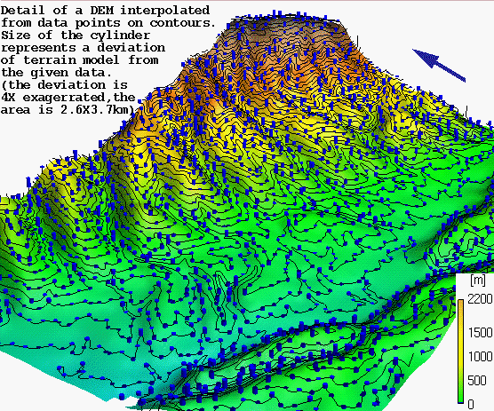
The RST variational capabilities proved to be very useful in our effort to prepare adequate inputs for simulations by enabling us to avoid the introduction of artificial features often produced by traditional interpolation methods (Mitasova and others, 1996; Mitasova and others, 1995b). Visualization plays an important role in detecting these artificial features (Wood and Fisher, 1993), which are often within acceptable accuracy but which distort the geometry of the surface/hypersurface, potentially leading to artificial patterns in the results of simulations. The role of visualization in detecting this type of errors is illustrated by interpolation of a high resolution digital elevation model (DEM) . While the standard 2D raster maps suggest an acceptable DEM quality for the most of the interpolation methods applied to the test data, viewing the results as surfaces with lighting and shading reveals serious distortions in surface geometries. By identifying deficiencies in interpolation techniques, visualization of interpolated fields as lighted/shaded surfaces in 3D space, rather than 2D contours or color raster maps, has contributed to the development of significant improvements in interpolation methods and algorithms (e.g., Mitasova and others 1995b, Wood and Fisher 1993).
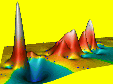
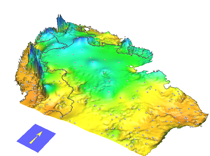
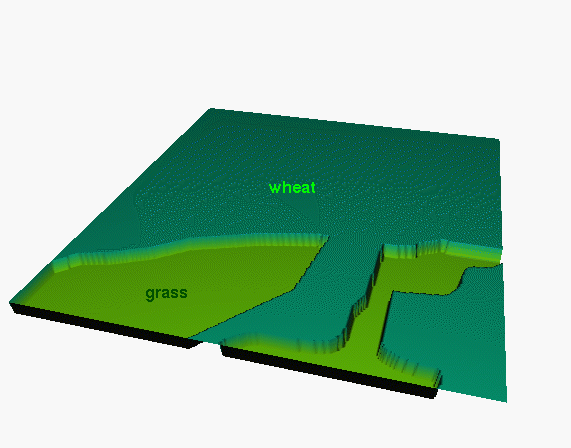
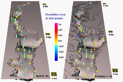
The use of dynamic cartographic models for visual analysis of multi-variate landscape phenomena characterized by sets of discrete sampling points and by interpolated surfaces/hypersurfaces is illustrated by examples in Table 1.. The possibility to visualize the data points in 3D space, fly through the point space, select certain values (e.g., time) as a third dimension and assign various graphical variables (size, color, shape, numerical label) to selected attributes (Brown, 1996b, Table 1: column 2), facilitates visual analysis of spatial relationships between the locations of point data and their measured values. The display of interpolated surfaces together with data points sized and/or colored according to the values of deviations or predictive errors was especially useful for evaluation of interpolation techniques used to generate the surfaces and for assessing the uncertainty of the resulting raster data sets (Table 1: elevation, concentration of chemicals in water). More complex approaches to the analysis and visualization of uncertainty were proposed, for instance, Ehschlaeger, Shortridge, and Goodchild (1997) and by Davis and Keller (1997). Visual analysis of multi-variate raster data (Table 1: column 3) is supported by capabilities to create animations with spatial change (key-frame animation for fly-by), as well as dynamic models with chronological or attribute change (DiBiase and others, 1992; MacEachren, 1994), by generating a series of images using scripting tools. Vertical relationships between multiple surfaces, typical for representation of soil data, are analyzed by moving cutting planes. Surface/hypersurface representation is not restricted to globally continuous fields. A method for effective representation and visualization of surfaces with discontinuities, using splines and GIS tools, was developed by Cox, Kohn, and Gleadow (1994). Phenomena represented by classes, such as vegetation or land use, can be represented as surfaces with faults (Table 1: land cover).
Table 1. Examples of landscape phenomena visualization using point symbols, dynamic surfaces and isosurfaces. Click on the image to retrieve a full size picture (approx. size 50-150K), or animation (approx. size 50-200K)
Visualization of landscape characterization data as multi-variate fields modeled by bi-, tri-, and quad-variate Regularized Spline with Tension | ||||
| phenomenon (field) | point data | 3D dynamic map | ||
|---|---|---|---|---|
| elevation: z=f(x,y) | |
|
||
| precipitation: pi=fi(x,y); i=1,...,12 | |
|
||
| soil horizons: zi=fi(x,y); i=1,...,5 | |
|
||
| soil texture: P=f(x,y,z), P={Sd}, d=20, 80, ... | |
|
||
| land cover: z+hi=fi(x,y), i=1,...12 | |
|
||
| underground concentrations of chemicals: w=f(x,y,z,t) |
|
|
||
| concentration of chemicals in water: w=f(x,y,z,t) | |
|
||
An adequate visual representation of continuous surfaces/hypersurfaces,
without visible patterns of their discrete raster representation,
was achieved by interpolating the input point data to rasters with
high resolutions, effectively describing the geometry of the modeled phenomena.
Perception of continuity was further enhanced by using Gouraud shading
(Hearn and Baker, 1986).
High resolution interpolation in the 4th (temporal)
dimension was important for animation of spatio-temporal
data, due to the fact that a meaningful dynamic cartographic model
requires gradual changes in the sequence of images used as
frames in animation.
Another important issue, illustrated by the examples in Table 1, is
scaling in the 3rd (vertical) and 4th (temporal) dimensions,
discussed in more detail by Brown and others (1995) and
Mitasova and others (1995a).
For many cartographic models, vertical spatial variability
requires resolutions much higher than the resolutions used for
the representation of phenomena in a horizontal plane.
Typically, a global vertical exaggeration factor is applied for better
visual perception of terrain, but we have also found that a
spatially variable, or relative vertical exaggeration is
often needed (Brown and Astley, 1995).
To visualize vertical relationships with sufficient detail,
relative exaggeration of depths was used both for multiple
surfaces representing the soil horizons (depths exaggerated relative
to terrain surface) and for the time series of volumetric data
representing chemical concentrations (Table 1).
A cube, stretched in the vertical dimension, was used as a scale
to represent a global or spatially constant exaggeration.
The efficiency and suitability of visualization tools for
exploring multi-variate land characterization data
is ensured by a high level of interactivity and by a
combination of advanced visualization capabilities
with the traditional spatial query and analysis functions
of a GIS (Brown and others, 1995; Brown and Astley, 1995).
In an effort to expand some of the interactive visualization
capabilities to users accessing the cartographic
models on the World Wide Web (WWW),
a simple translator of georeferenced raster data to
Virtual Reality Modeling Language
(VRML) format files, has been developed. This translator,
implemented in a GIS as the command
p.vrml (Brown, 1996a),
can be used
to output the models of landscape phenomena stored in a GIS
data base as VRML format files, enabling sharing of surface visualizations
on the WWW. To illustrate the current functionality and limitations
of this capability, a digital elevation model draped with a raster map
representing spatial distribution of erosion/deposition was
transformed to VRML representation.
(VRmodel 1).

Currently, VRML is not well suited for large data sets which can result from even a small geographic region. For reasonable file size and interactivity, the resolution and dimensions of the presented example have been reduced, compared to the resolution used for the actual modeling and visualization within a GIS (Movies 1, 2, 3, 4).
The VRML translator will be enhanced to allow precise setting of multiple viewpoints, additional data types (point and vector data), legends, and embedded WWW links associated with specific objects or locations in the model. A good example of the use of such hyperlinks, as well as types of cartographic symbols being used in VRML, is the Maui "world" produced by the SAVE Maui Program. The translator will also be upgraded to use the VRML 2.0 specification, which will be much more efficient for geographic applications, as it introduces an "ElevationGrid" node so that only the elevation points will have to be written instead of the whole geometry, greatly reducing file size and, more importantly, allowing VRML browser developers to use this information to enable faster drawing and more meaningful interaction.
Because the VRML specification allows for event-driven change in the
model, it may become an appropriate visualization method for
viewing and guiding a dynamic model (DiBiase, 1990).
Further investigation is necessary to determine how practical such an application
might be.
To elucidate the role of exploratory cartographic visualization in the process of development, application and communication of landscape simulations, we use the example of a distributed process-based erosion model SIMWE (SIMulation of Water Erosion), developed to support the design of effective erosion prevention measures.
The SIMWE erosion model is based on the solution of the continuity equation which describes the flow of sediment over the landscape, depending on a steady state water flow, detachment and transport capacities and properties of soil and cover, as explained in more detail by Mitas and others (1996) and by Mitas and Mitasova (manuscript in preparation). Net erosion/deposition D(r) at a point r=(x,y) is estimated as a divergence of a vector field q(r) representing sediment flow:
(1)
under the assumption that the erosion and deposition are proportional to the difference between the sediment transport capacity T(r) and the actual sediment flow rate q(r) (Foster and Meyer, 1972):
(2)
where C(r) is the first order reaction coefficient dependent on soil and cover properties. We solve the continuity equation in a modified form:
(3)
where p(r) =|q(r)|/|v(r)|, v(r) is the water flow velocity, and d is the diffusion constant. The equation (3) is solved by a stochastic method which provides the robustness necessary for handling rapid changes in input fields, especially in land cover, often caused by human intervention. Results of the model depend on the interaction between the input fields, especially the soil transport and detachment capacities and actual sediment loads and detachment rates. These interactions are complex and even small changes in the input fields can have a dramatic impact on the resulting prediction of erosion/deposition. Use of multiple dynamic surfaces and moving cutting planes provides an insight into the underlying differential equation solution and into the model behavior, as illustrated in more detail by the following examples of application to an experimental farm of the Technical University Muenchen, Germany (Auerswald and others, 1996).
The sediment flow equations are solved by a Green's function Monte Carlo method (Schmidt and Ceperley, 1992; Kalos and Whitlock, 1986; Mitas, 1996) which is based on sampling the solution(s) of equation (3a,) using a stochastic process which corresponds to the underlying differential equation (Gardiner, 1985). By accumulating a sufficient number of samples, one estimates the actual sediment concentrations with an error inversely proportional to the square root of number of samples. The process of solution is illustrated by two dynamic surfaces. The first surface and its color represent the distributions of sediment flow rates |q(r)| obtained as solutions of the differential equation (3). The second surface represents actual terrain with predicted erosion/deposition rates D(r) draped as a color map. Number of samples, a parameter in the method of solution, is used as the "temporal" variable for the animation. Increasing the number of samples decreases the roughness of the sediment flux surface and consequently reduces the noise in the erosion/deposition map (Movie 1). This process can also be interpreted as a process of reducing the statistical error of the solution of the differential equation (3), with the roughness in the first surface and the noise in the second surface representing the measure of statistical uncertainty. It is important to distinguish between the use of Monte Carlo as a method for solving differential equations and Monte Carlo applications to uncertainty or error propagation studies, such as the application by Davis and Keller (1997). In studies of uncertainty, a set of samples with a random component is generated to evaluate the likelihood of possible scenarios, the distribution of quantities which are compatible with the given data, or the impact of errors in subsequent processing. The presented approach is different: we generate samples of a unique solution of the second order differential equation (3) using a projection (Green's function) method. The projection can be carried out by a variety of techniques, for linear cases, Monte Carlo is one of them. In the limit of infinite number of samples (zero statistical error) the estimator will be identical to the exact solution of the equation (3).


The animation shows that a relatively modest sampling is sufficient to provide a useful estimate of main features of sediment flux distribution, while more sampling is needed for an adequate erosion/deposition map, where the computation of divergence is sensitive to the noise in the sediment flux surface. Draping color on terrain highlights the relation between the erosion/deposition and terrain shape and shows higher sensitivity to the noise on hillslopes with low values of sediment flux, while major erosion features in valleys are predicted using a relatively small number of samples. The animation was created using the NVIZ visualization program (Brown and Astley, 1995), and by automatically displaying and saving a series of images representing the solutions obtained with a gradually increasing number of samples (from 75,000 up to 50 million). The series of images was then transformed to the mpeg movie.
The spatial distribution of erosion and deposition is influenced by the first-order reaction coefficient C which reflects the detachment and transport properties of soil. To gain an insight into the role of this parameter we performed simulations for the C values uniformly changing over several magnitudes, resulting in a series of raster maps representing spatial distributions of sediment flux and erosion/deposition for soils with gradually increasing particle size (Movie 2). As in the previous example, we have simultaneously animated sediment flux (surface and color) and terrain with simulated erosion/deposition draped as a color map.

To evaluate the capability to correctly predict the location of areas with potential for deposition, the model results were compared with the observed depths of colluvial deposits. For visual comparison, we have displayed 3 relevant surfaces with a color map, and used a moving cutting plane to analyze their horizontal and vertical spatial relationships. The three surfaces represent terrain, maximum depth of colluvial deposits (elevation minus the thickness of colluvial deposit), and a reference plane used to enhance the 3D visual perception. Results of the erosion/deposition model were draped over the terrain surface as a color map. A series of images was then created and animated by cutting the surfaces by a vertical plane moving at a given interval from north to the south, allowing us to view the observed depth of colluvial deposits and compare it to the colors draped over the terrain surface (Movie 3). While we found good agreement between the observed and predicted location of deposition in the concave parts of the hillslopes and valleys, there was also a part of a rather steep, convex hillslope with a relatively thick layer of observed deposits, where the model predicted significant erosion. Further investigation of the land use in the study area provided explanation for the unusual location of deposition, which was due to the long term dense grass cover in this part of the hillslope which captured the soil eroded from the neighboring agricultural areas (Mitas and others, 1996).

An important application of erosion modeling is to evaluate the consequences
of land use change and support improvements in land use management to
achieve maximum land use with a minimum negative impact of erosion/deposition.
In our study area, we used the erosion model
for the evaluation of various distributions of protective grass cover aimed at
finding its more effective spatial distribution
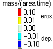
while keeping the percentage of grass cover at the current level (30%)
(Fig. 3A). With the current location of grass,
there is still a significant amount of sediment delivered
to the stream (Fig. 3B) with a strong potential of creating rills and
gullies (Fig. 3C, dark red areas).
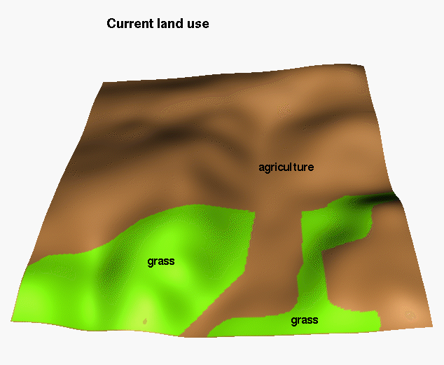
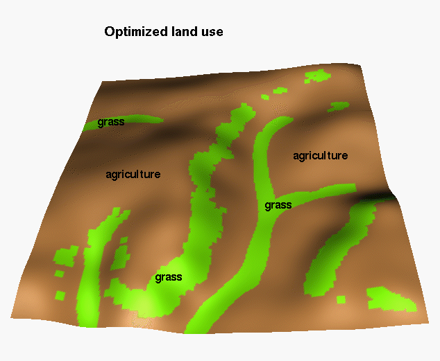
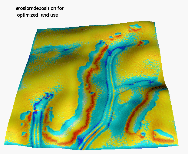
Redesigning the land use so that the protective grass cover
is located in the highest erosion risk areas (Fig. 4A)
can dramatically reduce soil loss and sediment delivery to
the streams (Fig. 4B,C).
Visualization in this case helps to understand the relationship
between the location of erosion protection measures and
terrain geometry and highlights the dramatic reduction of sediment
flow by implementing protective grass stripes (Fig. 3B, 4B).
The process of finding the effective spatial distribution of grass
is illustrated by Movie 4, which distributes grass to areas where the
treshold of maximum acceptable erosion/deposition rate is decreasing from
1.0 to 0.001 mass/area.sec.
This animation confirms, that to prevent
erosion and high sediment loads in streams, it is important to protect
higher, convex parts of hillslopes, rather than just widening
the buffers along the streams in valleys.
 A
A
 B
B
 C
C
 A
A
 B
B
 C
C

We have presented a series of applications which elucidate the role of exploratory cartographic visualization in the development and presentation of models of landscape phenomena and processes. The models are based on a multi-variate fields representation and description of processes by first principles equations. The visualization of landscape characterization data demonstrated the use of dynamic cartography as a data exploration tool. The role of cartography, at various stages of simulation tools development, was illustrated by animations representing the method of solution, the influence of model parameters, the comparison of model results with field data, and the improvement of erosion protection measures. These examples demonstrate the extension of modern computer cartography from a tool for automatization of paper map production towards providing methods and techniques aimed at exploration and communication of complex georeferenced data and their spatial and spatio-temporal relationships.
Further development
and wider applications of the presented cartographic visualization techniques
will be driven by full integration of multi-dimensional data structures
and their support within GIS, by larger volumes of spatio-temporal
data available and by improvements in speed and quality of graphics
on personal computers (at least to the level now available
only on graphical workstations).
While visualization cannot and does not solve the landscape simulation
problems which require improvement of algorithms and extensive
field experiments for calibration,
it plays an important role in understanding landscape processes
and their models and helps to narrow the path to solutions.
This provides strong
motivation for wide usage and further development
of the presented techniques, especially
for tasks related to environmental modeling and management of
natural resources.
Acknowledgments-
This project was funded in part by the Strategic Environmental Research
and Development Program (SERDP).
We greatly appreciate the continuing support from the USA Construction
Engineering Research Laboratories (USA CERL) and the possibility to
use computational resources at the
National Center for Supercomputing Applications (NCSA) in Urbana-Champaign, IL.
L. Mitas is partially supported by the
DARPA Grant DABT63-95-C-0123 .
We would also like to acknowledge the contribution of data by
the USA CERL, Prof. K. Auerswald
(Technical University Muenchen, Germany) and Dr. S. Warren
from USA CERL, L.A.K. Mertes, Department of Geography, University
of California Santa Barbara, and EPA, Chesapeake Bay monitoring program.
Auerswald, K., A. Eicher, J. Filser, A. Kammerer, M. Kainz, R. Rackwitz, J. Schulein, H. Wommer, S. Weigland, and K. Weinfurtner, 1996, Development and implementation of soil conservation strategies for sustainable land use - the Scheyern project of the FAM: in Stanjek, H., ed., Development and Implementation of Soil Conservation Strategies for Sustainable Land Use, Int. Congress of ESSC, Tour Guide, II, Technische Universitat Muenchen, Freising-Weihenstephan, Germany, p. 25-68.
Brown, W.M., 1996a, VRML translator for GRASS4.2: p.vrml ,
Geographic Modeling and Systems Laboratory,
University of Illinois at Urbana-Champaign.
http://www.cecer.army.mil/grass/viz/pvrml.man.html
Brown, W.M., 1996b, SG3d - supporting information. Enhancements for GRASS4.2:
Geographic Modeling and Systems Laboratory,
University of Illinois at Urbana-Champaign.
http://www.cecer.army.mil/grass/viz/sg3d42.html
Brown, W.M., and Gerdes, D.P., 1992, SG3d - supporting information:
U.S. Army Corps of Engineers, Construction Engineering Research Laboratories,
Champaign, Illinois.
http://www.cecer.army.mil/grass/viz/sg3d.html
Brown, W.M., and Astley, M., 1995,
NVIZ tutorial: Geographic Modeling and Systems Laboratory,
University of Illinois at Urbana-Champaign.
http://www.cecer.army.mil/grass/viz/nviz.tut.html
Brown, W.M., Astley, M., Baker, T., and Mitasova, H., 1995, GRASS as an integrated GIS and visualization environment for spatio-temporal modeling: Proceedings Auto-Carto 12, Charlotte, NC, p. 89-99.
Cox, S., Kohn, B.P., and Gleadow, A.J.W., 1994,
Towards a fission track tectonic image of Australia: model based
interpolation in the Snowy Mountains using a GIS:
http://www.ned.dem.csiro.au/AGCRC/papers/snowys/12agc.cox.html
Davis, T. R. and Keller, C. P., 1997, Modelling multiple spatial uncertainties: Computers and Geosciences, this issue.
DiBiase, D., 1990, Visualization in the Earth Sciences: Earth and Mineral Sciences, v.59, no. 2, p. 13-18.
DiBiase, D., MacEachren, A.M., Krugier, J.B., and Reeves, C., 1992, Animation and the role of map design in scientific visualization: Cartography and GIS, v. 19, no. 4, p. 201-214.
Ehlschlaeger, C. R., Shortridge, A. M., and Goodchild, M. F., 1997, Visualizing spatial data uncertainty using animation: Computers and Geosciences, this issue.
Ervin, S. M., 1993, Landscape visualization with Emaps: IEEE Computer Graphics and Applications: v. 13, no. 2, p. 28-33.
Fisher, P., Dykes, J., and Wood, J., 1993, Map design and visualization: The Cartographic Journal, v. 30, no. 12, p. 136-142.
Foster G R, Meyer L D 1972 A closed-form erosion equation for upland areas: Shen, ed., Sedimentation: Symposium to Honor Prof. H.A.Einstein: Colorado State University, Ft. Collins, CO, p.12-1.-12-19.
Gardiner, C.W., 1985, Handbook of stochastic methods for physics, chemistry, and the natural sciences: Springer, Berlin, 462 p.
Hargrove, W., Hoffman, F., and Levine, D., 1995, Clinch river environmental restoration program: http://www.esd.ornl.gov/programs/CRERP/
Hearn, D., and Baker, M.P., 1986, Computer graphics: Prentice-Hall, Inc., Englewood Cliffs, New Jersey, p. 289-291.
Hibbard, W. L., and Santek, D.A., 1989, Visualizing large data sets in the earth sciences: Computer, v. 22, no. 8, p. 53-57.
Hibbard W.L., Paul B.E., Battaiola A.L., Santek D.A.,
Voidrot-Martinez M-F., and Dyer C.R., 1994,
Interactive Visualization of Earth and Space Science Computations:
Computer v. 27, no. 7, p. 65-72.
http://www.ssec.wisc.edu/~billh/vis.html
Kalos, M. H., and P. A. Whitlock, 1986, Monte Carlo methods: J. Wiley, New York, 225 p.
Kennie, T. J. M., and McLaren, R. A., 1988, Modelling for digital terrain and landscape visualization: Photogrammetric Record, v.12, no. 72, p. 711-745.
Kraak, Menno J., 1993, Cartographic terrain modeling in a three dimensional GIS environment: Cartography and Geographic Information Systems, v. 20, co. 1, p. 13-18.
MacEachren, A.M., and Ganter, J.H., 1990, A pattern identification approach to cartographic visualization: Cartographica, v. 27, no. 2, p. 64-81.
MacEachren, A.M., 1994, Time as cartographic variable: in Hearnshaw, H.M., and Unwin, D.J., ed., Visualization In geographical Information Systems: John Wiley and Sons, Chichester, p. 115-130.
Mitas, L., 1996, Electronic structure by Quantum Monte Carlo: atoms, molecules and solids: Computer Physics Communications, v. 97, p. 107-117.
Mitas, L., and Mitasova, H., 1988, General variational approach to the interpolation problem: Computers and Mathematics with Applications, v. 16, no. 12, p. 983-992.
Mitas L., Mitasova H., Brown W. M., and Astley M., 1996 ,
Interacting fields approach for evolving spatial phenomena:
application to erosion simulation for optimized land use:
Proceedings of the III. Int. Conf. on Integration of Environmental Modeling
and GIS (Santa Fe, NM), by National Center for Geographic Information
and Analysis, Santa Barbara CA, CD ROM and WWW.
http://www.cecer.army.mil/grass/viz/SF.final/mitas.html
Mitasova, H., and Mitas, L., 1993, Interpolation by Regularized Spline with Tension: I. Theory and implementation: Mathematical Geology, v. 25, no. 6, p. 641-655.
Mitasova H., Brown W.M., and Hofierka J., 1994, Multi-dimensional dynamic cartography: Kartograficke listy, v. 2, p. 37-50.
Mitasova, H., Mitas, L., Brown, W.M., Gerdes, D.P., Kosinovsky, I., and Baker, T., 1995a, Modeling spatially and temporally distributed phenomena: new methods and tools for GRASS GIS: International Journal of Geographical Information Systems, v. 9, no. 4, 433-446.
Mitasova, H., Brown, W.M., Johnston, D.M., Saghafian, B., Mitas, L., and Astley, M., 1995b, GIS tools for erosion/deposition modeling and multidimensional visualization. Part I: Interpolation, Rainfall-runoff, Visualization: Report for USA CERL, University of Illinois at Urbana-Champaign, IL, p. 45.
Mitasova, H., Hofierka, J., Zlocha, M., and Iverson, L.R., 1996, Modeling topographic potential for erosion and deposition using GIS: Int. Journal of GIS, v. 10, no. 5, p. 629-641.
Moellering, H., 1978, A Demonstration of the Real Time Display of Three Dimensional Cartographic Objects: computer generated video tape, Department of Geography, Ohio State University.
Moellering, H., 1980, The Real-Time Animation of Three Dimensional Maps: The American Cartographer, v. 7, no. 1, p. 67-75.
Monmonier, M., 1990, Strategies for the visualization of geographical time series data: Cartographica, v. 27, no. 1, p. 30-45.
Nielson, G. M., Foley, T. A., Hamann, B. and Lane, D., 1991, Visualizing and modeling scattered multivariate data: IEEE Computer Graphics and Applications, v. 11, no. 3, p. 47-55.
Openshaw, S., Waugh, D. and Cross, A., 1994, Some ideas about the use of map animation as a spatial analysis tool: in Hearnshaw, H.M., and Unwin, D.J., ed., Visualization In geographical Information Systems: John Wiley and Sons, Chichester, p. 131-138.
Raper, J. (ed.), 1989, Three Dimensional Applications in Geographical Information Systems: Taylor and Francis, London, p. 254.
Rhyne, T., Bolstad, M., Rheingans, P., Petterson, L., and Shackelford, W., 1993, Visualizing environmental data at the EPA: IEEE Computer Graphics and Applications, v. 13, no. 2, p. 34-38.
Saghafian B., 1996, Implementation of a Distributed Hydrologic Model within GRASS: in Goodchild, M.F., Steyaert, L.T. and Parks, B.O., eds., GIS and Environmental Modeling: Progress and Research Issues, GIS World Inc., p. 205-208.
SAVE Maui Program, 1996, Maui World http://nko.mhpcc.edu/pavillion.html
Schmidt, K. E., and Ceperley, D. M., 1992, Monte Carlo Techniques for Quantum Fluids, Solids and Droplets: Binder, K., ed., Monte Carlo Methods in Statistical Physics III, Springer, Berlin, p. 205-248.
Slocum, T.A., 1994, Visualization software tools: in MacEachren, A.M., and Taylor, D. R. F., eds., Visualization in Modern Cartography, Pergamon, Elsevier Science Ltd, London, p. 91-94.
Stephan, E.M., 1995, Exploratory data visualization of environmental data for reliable integration: Proceedings Auto-Carto 12, Charlotte, NC, p. 100-109.
Wood, J. D., Fisher, P. J., 1993, Assessing Interpolation Accuracy in Elevation Models: IEEE Computer Graphics and Applications, v. 13, no. 2, 48-56.
Tobler, W., 1970, Computer movie simulating urban growth in the Detroit region: Economic Geography, v. 46, p. 234-240.
Yarrington, L., 1996, Fernald geostatistical techniques: Sandia National Laboratory, NM. http://www.nwer.sandia.gov/fernald/techniq.html