 GMSL Modeling & Visualization Home Page
GMSL Modeling & Visualization Home Page
Spatial Modeling and Systems Team
U.S. Army Construction Engineering Research Laboratories
P.O. Box 9005
Champaign, IL 61826-9005, USA
and
GIS Laboratory
University of Illinois at Urbana-Champaign
220 Davenport Hall, Urbana, IL 61801, USA.
Increasingly, geoscientific data is being measured in three dimensional (3D) space and time for studies of spatial and temporal relationships in landscapes. To support the analysis and communication of these data, a new approach to cartographic modeling is emerging from the integration of computer cartography and scientific visualization. This approach, which we call in this paper multidimensional dynamic cartography (MDC), is based on viewing data processed and stored in a Geographical Information System (GIS) in 3D space and visualizing dynamic models of geospatial processes using animation and data exploration techniques. Such techniques help researchers refine and tune the model in addition to making the model easier for others to understand. We describe various aspects of MDC implementation within GRASS GIS and illustrate its functionality using example applications in environmental modeling. Images, animations and other work associated with this paper may be viewed on the World Wide Web at URL: http://www.cecer.army.mil/grass/viz/VIZ.html
Current standard GIS offer sophisticated tools for creating high quality cartographic output in the form of standard 2D maps. While such maps fulfill the requirements of GIS as an information retrieval and maintenance system, they are not adequate for application of GIS as a tool for analysis of spatio-temporal data and simulation of landscape processes which occur in 3D space and time. (McLaren 1989). To support such applications, GIS has been linked to various visualization systems. However, such links require the user to learn two different environments - one for processing the data and a second one for visualization. To increase efficiency and convenience for the researcher in using visualization for routine modeling and analytical work we have chosen to build visualization tools within GIS and design them to fulfill specific needs of geoscientific data.
Three levels of GIS and visualization integration are defined by (Rhyne 1994): rudimentary, operational and functional. The rudimentary level is based on data sharing and exchange. The operational level provides consistency of data and removes redundancies. The functional form provides transparent communication between the two software environments. We would add that at the functional level, data manipulation and derived data from visualization should be able to be written back to the GIS as new data layers, so that visualization can be used for data development.
Our MDC environment, integrated at the operational level, uses GIS to easily do transformations between coordinate systems, manage spatial data, run simulations, and derive statistical or other visually meaningful layers such as cross validation error or profile convexity (Wood 1993). The visualization tools use known characteristics of geographic data types to speed data exploration algorithms and provide more meaningful responses to interactive data queries. Customized visualization techniques are incorporated to meet common needs of researchers doing cartographic modeling.
An integrated approach also encourages verification of modeled scenarios with actual measured data by providing a common computational/display environment. Well tested models developed in this way are less likely to be dataset-specific because it should be easier to test the model with a variety of datasets under various geographic conditions.
MDC may be thought of as a special case of scientific visualization; while more confining as to its requirements of data types (to conform to types supported by the GIS), MDC offers a specialized palette of data manipulation and viewing tools and symbolic representations that are meaningful to cartographers.
MDC can be used as either a process of research and discovery or a method of communicating measured or modeled geographic phenomena. As a process of discovery, the MDC process is cyclical in nature, with visualizations feeding a refinement of the model. As a method of communication, MDC is used to demonstrate complicated processes through the use of images and animations.
Combinations of various graphical representations of raster, vector, and point data displayed simultaneously allow researchers to study spatial relations in 3D space. At the same time, visual analysis of data requires the capability to distort this spatial relation by changing vertical scale, separating surfaces, performing simple transformations on point or vector data for scenario development, etc.
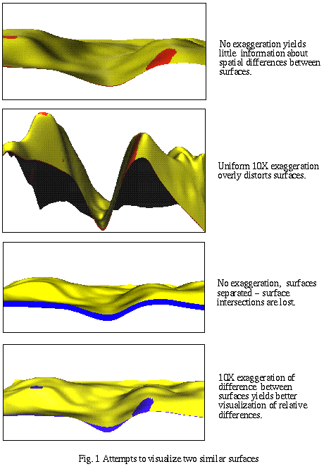
Multiple surfaces are quite useful to visualize boundaries of layers. For example, surfaces may be created that represent soil horizons so that thickness of layers may be displayed. This presents a technical challenge in terms of dimensional scale, as demonstrated by figure 1. The vertical dimension is often quite small relative to the other two, so is often exaggerated when a single surface is displayed. This exaggeration is usually adequate to add relief to an otherwise featureless surface, but in order to separate close stratified layers, the required exaggeration grossly distorts the modeled layers. If vertical translation of a surface is used to separate surfaces enough that they may be viewed separately, intersections between surfaces and relative distances are misrepresented. This is unacceptable since these may actually be the features we are interested in viewing. To study differences between two similar surfaces, we use a scaled difference approach where only the spatial distance between surfaces is exaggerated, maintaining correct surface intersections.
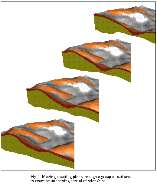
Animation is an important tool for exploring large and complex data sets, especially when they involve both spatial and temporal dimensions. Recent progress in graphics technology and emerging standards for animation file formats have made desktop animations easier to produce and share with colleagues. Animation is useful for representation of change in time, change in a modeling parameter (Ehlschlaeger 1994), change in viewer position (fly-bys) or change in visible data (fence cuts, slices). Figure 2 shows several frames from an animation where a fence cut is moved through data to better view underlying surface structure.
General Description
GRASS (Geographic Resources Analysis Support System) as an open, public domain system with a full range of GIS capabilities has provided a sound basis for testbed development of visualization tools for MDC. Each GRASS data type (raster, vector, and site) plus our own 3D grid format may be used for visualization in a single 3D space. In our implementation, there are four object types and various ways to represent each.
Surfaces. A surface requires at least one raster data set to represent topography and may use other raster data sets to represent attributes of color, transparency, masking, and shininess. These data sets may have been derived from vector (e.g., countour) or scattered point data using tools within the GIS. Users are allowed to use a constant value in the place of any raster data set to produce, for example, a flat surface for reference purposes or a constant color surface.
Vector sets. 3D vector sets are not currently supported, so in order to display 2D vector sets in 3 dimensions, they must be associated with one or more surfaces. The 2D vector sets are then draped over any of these surfaces.
Site Objects. Point data is represented by 3D solid glyphs. Attributes from the database may be used to define the color, size, and shape of the glyphs. 2D site data must be associated with one or more surfaces, and 3D site data may be associated with a surface (e.g., sampling sites measured as depth below terrain).
Volumes. 3D grid data may be represented by isosurfaces or cross sections at user-defined intervals. Color of the isosurfaces may be determined by threshold value or by draping color representing a second 3D grid data set over the isosurfaces.
For interactive viewer positioning, scaling, zooming, etc., we use custom GUI widgets and a "fast display mode" where only wire mesh representations of the data are drawn. When rendering a scene, the user may select various preset resolutions for better control over rendering time. For positioning we also chose to use a paradigm of moving viewer rather than moving object because we think it is more intuitive when modeling a reality of generally immobile geography. To focus on a particular object, the user simply clicks on the object to set a new center of view.
Scripting is used to create animations from series of data (e.g. time series or a changing modeling parameter), automatically loading the data sets and rendering frames for the animation. A keyframe technique is used to generate animations when there is no change in data, e.g., to create fly-bys or show a series of isosurfaces in volumetric data.
Interface
In addition to providing the functionality necessary for viewing various forms of data, it is also necessary to provide a usable front-end. In particular, we require the following features:
To satisfy these requirements our current interface is being developed using the Tcl/Tk toolkit written by John K. Ousterhout, and available via anonymous ftp. Tcl/Tk is an X windows based scripting and widget environment built on Xlib. Tcl/Tk provides a standard library of common widgets such as menus, buttons and the like, as well as a mechanism for developing arbitrarily complex custom widgets. Moreover, Tcl/Tk provides a natural mechanism for extension by allowing the creation of new commands via scripts or C code. Using this mechanism, we have incorporated our visualization library as an extension to Tcl/Tk. Thus, user's have access to visualization tools at the Tcl/Tk level, as well as the ability to extend Tcl/Tk with custom code.
Graphics Library
GRASS is designed to use various output devices for graphic display, via use of a display driver. The most commonly used is the X driver, for output to any X Window System display device. The GRASS driver interface is not currently capable of using 24-bit "true color" mode, as it was originally designed for display of a limited number of grid category values as a pseudocolor raster image. The GRASS driver only supports a limited set of graphic primitives, and only for a two dimensional, flat screen. While it is possible in such a system to display 3D objects and surfaces using a perspective projection, as was implemented in d.3d (USACERL 1993), all projection calculations have to be done explicitly and it is impossible to take advantage of specialized accelerated graphics hardware. Therefore we chose to use a separate display mechanism for visualization.
Fast graphics are required for effective interactive use of MDC. These graphics capabilities were identified early on as being integral in the development of MDC tools:
As our work progressed into rendering multiple surface and volume data, we identified these additional capabilities that are highly desirable:
For our early tools we used IRIS GL, a software interface specific to Silicon Graphics hardware which took full advantage of hardware acceleration to provide the required functionality and offered an easy-to-use programmers' interface.
As the importance of hardware acceleration for common 3D graphics calculations is being recognized by more hardware vendors, standard software interfaces become necessary in order to increase portability of software and standardize expected rendering behavior. Two such standards are the PHIGS extension to X (PEX), and OpenGL. While PEX is a library, OpenGL is a specification for an application programming interface (API)(Neider 1993). As such, it is up to each hardware vendor to provide an implementation of OpenGL which takes advantage of proprietary hardware acceleration. For current development we chose to use OpenGL and GLX, the OpenGL extension to X, partly because of the ease of porting IRIS GL to OpenGL (enabling re-use of earlier software development) and partly because of our impression that OpenGL implementations would be more likely to provide superior performance on a wide variety of platforms.
Computer Memory Considerations
Environmental data sets are very large, often involving several million data values for a single time step (Rhyne 1993). In order to effectively interact with this data, much of it needs to be loaded into computer memory to make access faster. The rendering process also adds additional memory overhead. During development of our tools, we tried to limit memory requirements for a typical application to 16-48 Mbytes, which is a common configuration for an average workstation.
In our implementation, 2D data sets are loaded into memory at the resolution defined by the user within the GIS. 3D data sets are not kept in memory, and the user may define whether specific vector or point data should be loaded into memory or read from the GIS whenever needed.
As an example, consider a simple 2D grid data set which is to be rendered as a surface with another 2D data set used for pseudocolor of the surface. In order to render a regular polygonal surface from this data, each data value will need to be located in 3D space by three coordinates with floating-point accuracy to represent a vertex of the surface. In order to simulate lighting, a three-component surface normal also needs to be calculated for each vertex. Assuming the data used to represent color is four byte data and floating point numbers occupy four bytes, the storage requirements for each surface vertex would be 28 bytes. So in the case of a 1000 X 1000 surface, we would already be using 28 Mbytes.
To reduce this requirement we can use known information about the data. Since we know the data represents a regular grid, with offset and resolution obtainable from the GIS, the east and west coordinates may be quickly calculated on-the-fly. We can interrogate the GIS to find the range and accuracy of the data and use the smallest data type possible to store the elevation and color of the surface. We could also calculate the surface normals on-the-fly, but the normals only change when the user adjusts resolution or exaggeration so we chose to pre-calculate and store surface normals to avoid repetitive calculations and speed rendering. However, we found through experimentation that the resolution of the surface normals could be reduced so that each normal may be stored in a single packed 4 byte field instead of three 4 byte floating point numbers. In the case of surface normals, we use 11 bits for each of the east and west components of the normal and 10 bits for the vertical component (taking advantage of our knowledge that a normal to a regular gridded surface will never be negative in the vertical component). Using these figures, the estimated requirements for a 1000 X 1000 surface reduce to 6-12 Mbytes.
When viewing multiple surfaces it is often common to use a data set more than once (perhaps topography for one surface and color for another). Our implementation shares data in such cases, freeing memory when a surface is deleted from the display only after checking that other surfaces aren't using the same data.
Mesh optimization was considered and rejected as a method of reducing memory requirements due to several conflicts: 1) In order to realistically render a mesh with widely varying polygon size, Phong shading is required for lighting calculations so that the surface normals are smoothly interpolated across the surface of each polygon. OpenGL only supports Gouraud shading, which interpolates color across the polygon from the color calculated at each vertex. 2) Draping 2D vector data on a surface requires finding the intersections of the vector lines with the edges of surface polygons. Using a regular mesh enables us to use faster intersection algorithms with less memory overhead. 3) In order to use a second data set for surface color, polygons of the optimized mesh would either have to be texture mapped, a feature fewer platforms support, or the two optimized meshes would need to be intersected, again a time consuming and overhead intensive process. 4) Use of an optimized mesh results in some degradation of data which is not easily quantifiable for accurate representation to the user.
Even using the lowest estimates, a surface that is 3000 X 6000 cells would require 108 Mbytes of main memory. So in practice, the user specifies a lower resolution and the data is automatically resampled by the GIS when loading. Given that the average workstation display only has about one million pixels, the whole data set at full resolution can not be completely displayed. Although there is an advantage to being able to browse the full data set, then zoom in on a small area at full resolution, in general we have found that users can be made aware of memory constraints and use the regular GIS display to either define a smaller region or reduce the resolution as necessary.
In the future we hope to explore the possibilities of using a surface with variable resolution. For example, a user could identify a region of special interest which would be drawn at full resolution within a broader region displayed at lower resolution.
Surface Querying
Querying a 2D data set displayed as a raster image can be thought of as a scale operation and a translation operation. When a user clicks on a pixel, the relative position in the image is scaled by the resolution of a pixel and the north and east offsets are added to obtain the geographical position. When displaying surfaces in 3D space with perspective, however, clicking on a pixel on the image of the surface really represents a ray through 3D space. The point being queried is the intersection of this ray with the closest visible (unmasked) part of one of the surfaces in the display.
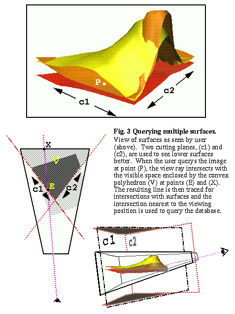
One method for 3D querying provided by OpenGL is a "selection" method, where objects are "redrawn" without actually drawing to the screen, and any objects drawn at the query point are returned as the "selected" objects. This method is slow and at best the returned object is a polygon rather than a specific point on the polygon. Therefore, we require the user to specify the type of data they are querying (surface, point, or vector) and then use our knowledge of the geometry of that data to perform a geometric query in 3D. Figure 3 shows that using cutting planes can allow the user to query a specific location on a surface that is covered by another surface.
This specialized point-on-surface algorithm can be outlined as follows:
Such point-on-surface functionality is useful for 3D data querying, setting center of view and setting center of rotation for vector transformations.
Examples of applications illustrating how a multidimensional dynamic approach to cartography increases its power for study of complex landscape processes are presented in a World Wide Web (WWW) document at http://www.cecer.army.mil/grass/viz/VIZ.html, accessible through Internet via browsers such as NCSA Mosaic. We have chosen to use the WWW to present and communicate applications of integrated GRASS GIS and visualization tools because of the opportunities to include full color images and animations which vividly illustrate the use of techniques discussed in this paper. The document covers several aspects of integration of GIS and visualization as they relate to applications in environmental modeling.
The first 3 documents ( "Surface Modeling", "Multidimensional Interpolation", and "3D Scattered Data Interpolation" ) represent modeling of spatial and spatio-temporal distribution of continuous phenomena in 2D and 3D space. Animations illustrate the properties of interpolation functions (Mitasova & Mitas 1993) used to transform the scattered site data to 2D and 3D rasters and show the difference between trivariate and 4-variate interpolation for modeling spatio-temporal distribution of chemicals in a volume of water (Mitasova et al. 1993).
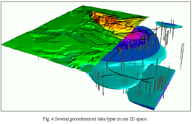
Animation based on changing data is illustrated by a dynamic surface representing change in monthly precipitation in tropical South America and by changing color map representing monthly temperatures on a static terrain surface in the same area. "Multidimensional Interpolation" also includes examples of a method for visualizing predictive error of interpolation along with the interpolated and animated surfaces using glyphs in data points. Images in "3D Scattered Data Interpolation" show the combination of all data types (2D, 3D raster, vector and sites), allowing users to study the spatial relationships between high chemical concentrations and terrain, railroads and wells (Fig 4). Animation is used to change the viewing position for better perception of spatial distribution of well sample sites in 3D space.
Terrain analysis and simulation of landscape processes related to fluxes of water and material are illustrated by "Terrain Analysis and Erosion Modeling" and "Rainfall Runoff" , which include dynamic surfaces and multiple dynamic surfaces representing waterflow accumulation, change in sediment transport capacity and results of hydrologic simulation (rainfall, runoff and infiltration)(Saghafian 1993). Use of multiple surfaces with animated cutting planes for modeling of soil geomorphology and for evaluation of an erosion/deposition model by comparing it with the measured depth of colluvial deposits is illustrated by "Soil Geomorphology".
All documents include references to manual pages and tutorials in experimental HTML form. References to scientific papers and ftp sites for software distribution are also included.
As the quantity of spatial data has grown in recent years due to more efficient data collection techniques such as remote sensing and Global Positioning Systems, GIS has played a vital role in managing this data. GIS capabilities such as user querying of data to obtain such metadata as coordinate system, scale and accuracy, or names of geographical features are sometimes taken for granted by modern cartographers, yet such features are often missing from generic modeling & visualization application programs.
When we speak of integration of GIS and scientific visualization, we are not talking about improved ways of accessing spatial data for visualization. Rather, we have identified opportunities for creating specialized custom visualization tools built for detailed analysis of georeferenced data. By integrating advanced visualization capabilities and modeling tools with the traditional spatial query and analysis functions of GIS, researchers are better able to evaluate a model's validity, explore possible causes of unexpected exceptions, tune modeling parameters, and re-visualize the results in a methodical, intuitive way.
This research was partially supported by the D.O.D. Strategic Environmental Research and Development Program, basic research, Digital Terrain Modeling and Soil Erosion Simulation.
Ehlschlaeger, C., Goodchild, M. 1994, Uncertainty in Spatial Data: Defining, Visualizing, and Managing Data Errors. Proceedings, GIS/LIS'94, pp. 246-53, Phoenix AZ, October 1994.
McLaren, R.A., Kennei, T.J.M. 1989, Visualization of Digital Terrain Models, Three Dimensional Applications in Geographic Systems, Jonathon Raper Ed. Taylor and Francis Ltd.
Mitasova, H., Hofierka, J. 1993, Interpolation by Regularized Spline with Tension: II. Application to terrain modeling and surface geometry analysis. Mathematical Geology, Vol. 25:657-669.
Mitasova, H., Mitas, Lubos. 1993, Interpolation by Regularized Spline with Tension: I. Theory and Implementation, Mathematical Geology, Vol. 25:641-655.
Mitasova, H., Mitas, L., Brown, W.M., Gerdes, D.P., Kosinovsky, I., Baker, T. 1993, Modeling spatially and temporally distributed phenomena: New methods and tools for Open GIS, Proceedings of the II. International Conference on Integration of GIS and Environmental Modeling, Breckenridge, Colorado
Neider, J., Davis, T., Woo, M. 1993, OpenGL Programming Guide, Addison-Wesley Publishing Co., Reading, MA Robertson, P.K. and Abel, D.J. 1993, Graphics and Environmental Decision Making IEEE Computer Graphics and Applications, Vol. 13 No. 2.
Rhyne, T. M., Bolstad, M., Rheingans, P. 1993, Visualizing Environmental Data at the EPA, IEEE Computer Graphics and Applications, Vol. 13 No. 2.
Rhyne, T. M., Ivey, W., Knapp, L., Kochevar, P., Mace, T., 1994, Visualization and Geographic Information System Integration: What are the needs and the requirements, if any ?, a Panel Statement in Proceedings IEEE Visualization '94 Conference, IEEE Computer Society Press, Washington D.C.
Saghafian, B. 1993, Implementation of a distributed hydrologic model within GRASS GIS. Proceeding of the II. International Conference on Integration of GIS and Environmental Modeling, Breckenridge, Colorado
U.S. Army Corps of Engineers Construction Engineering Research Laboratories 1993, GRASS 4.1 Reference Manual, Champaign, Illinois
Wood, J.D., Fisher, P.J. 1993, Assessing Interpolation Accuracy in Elevation Models IEEE Computer Graphics and Applications, Vol. 13 No. 2.